Back-Prop wo Calc

See below.

The Calculus you need to know

I explain a little bit about what calculus actually means in the Loss Landscape section, but I will briefly repeat it here.

You have a function $f$ which describes some relationship of change between two variables, illustrated:

$$y=f(x)$$

Where $x$ is the input variable, and $y$ is the output variable. I will also use $g$ later on to describe a second function.

“Doing Calculus”, also known as “Differentiating”, tells you how fast one variable is changing, with respect to (wrt), another variable. If the original function gives us a “shape” or curve of how to variables change wrt each other, differentiating gives us the Gradient of how they change wrt each other. This is the ”Gradient” of ”Stochastic Gradient Descent”.

Power Law

The most basic rule you will need. Say we have some function $f(x)=x^2$ that we want to differentiate, with respect to x (explanation for what that means in practical terms later on):

$$\frac{\partial f}{\partial x}=2x$$

What happens here, is the with respect to x to take the power rule, so

$$f(x)=x^y\to \frac{\partial f}{\partial x}=y{x}^{y-1}$$

We don’t care about the $y$ because we are only trying to differentiate for $x$. The $y$ is basically any variable or number which isn’t $x$. It follows that any differentiation that happens to any $y$ that isn’t multiplied or part of a power of $x$ simply goes to $y\to 0$. So for $f(x)=x+y$ :

$$\frac{\partial f}{\partial x}=1+0$$

I.e. the $x\to 1$ while the $y\to 0$.

So wait why did the $x\to 1$? So fun fact, $x$ is the same thing as $x^1$:

$$x=x^1$$

So if we apply the power rule to it:

$$1\cdot x^{1-1}\to x^0=1$$

So if you have something like $f=yx$ then $f^{\prime }=y\cdot 1$, or $f=2x$ then $f^{\prime }=2\cdot 1$. By the way, $f^{\prime }$ is the same thing as $\frac{\partial f}{\partial x}$ just written differently (“prime notation”).

A similar math identity to use before you differentiate with the power rule is:

$$\frac{1}{x}=x^{-1}$$

Use this to your advantage.

The Chain Rule

Ok so what about if we have a function inside another function. Say like an activation function in our neural network, which is dependent on the activation functions of other neurons. If $f(g(x))$ for the functions $f$ and $g$ we can apply the chain rule:

$$\frac{\partial f(g(x))}{\partial x}=\frac{\partial g(x)}{\partial x}\frac{\partial f(x)}{\partial g(x)}$$

This look complicated buy you have already seen it. In $f(x)=(x{)}^y$ you could say the $x$ is the function $g(x)=x$, and the $(\text{textunderscore}{)}^y$ is $f(g)=(g{)}^y$. So :

$$\frac{\partial f}{\partial g}=g^{\prime }\cdot y(g{)}^{y-1}$$

(I’m dropping the “(x)” here so it’s easier to type, I also used “prime notation” to represent the differentiation of $g$) This is the exact same as the previous equation. We swap in the function $g(x)=x$ and thus:

$$\frac{\partial f}{\partial x}=\frac{\partial }{\partial x}x\cdot y(x{)}^{y-1}\to 1\cdot y{x}^{y-1}=y{x}^{y-1}$$

---

I am going to illustrate this again, but with a new function $a_2=a_1\cdot w_{12}$ which we can say is the activation function of one layer, which is given by the activation value of the previous layer times the weight. But, that activation value of the previous layer is given to you by the activation function $a_1=a_0\cdot w_{01}$ and we want to derive with respect to $w_{0}1$, this gives us the chain rule:

$$\frac{\partial a_2}{\partial w_{01}}=\frac{\partial a_1}{\partial w_{01}}\frac{\partial a_2}{\partial a_1}=a_0\cdot w_{12}$$

Then, because you want to only describe this in terms of weight, replace whatever activation functions are left in terms of the weight where possible. For deriving the weight gradients at deeper layers, continue “nesting”, differentiating wrt each activation functions as needed.

---

The benefit of this is, you can nest derivations. Which will be useful when we want to see how a weight should change in comparison to the Cost (the amount of error) the network gets on an output, but because each layer is dependent on the activations and weights of the ones that came before it, we derive the function with respect to each of the activation functions along the chain of connected neurons, until we come to the weight we want to update. It also means we can reuse derivations from each layer moving backwards.

The calculus as you need as simple as I can put it

Derivation of the cost function

For Square-Error: $C={\left(a-y\right)}^2\to$

$$\frac{\partial C}{\partial a}=2(a-y)$$

Derivation of a ReLU Activation Function

WRT the weight. When wrt the activation, the result uses the same method, the power rule, but gives a different result. ReLU: $a_{currentlayer}=a_{previouslayer}\cdot w_{previoustocurrent}$ as long as output is greater than zero.

$$\frac{\partial a_{current}}{\partial w}=a_{previous}$$

The Chain Rule

Nope. You gotta read the above and then a few Wikipedia and Stack Exchange pages. Really not that hard.

A Simple Chain Network & Cost Function

Describing the Network and how we train it

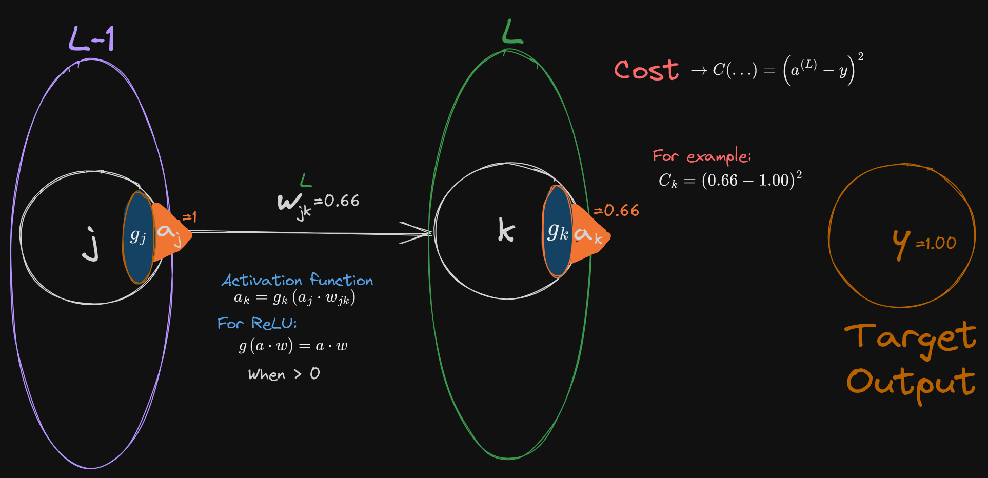
We describe the simplest possible model: Two units, an input node and an output node, connected by a single weight. We let the activation on the first node be the input value from the sample, so not a ReLU unit (sorry I know it shows an activation function in the drawing, but I’m not redoing it because we need it later ) this is connected directly to the output layer. This does contain ReLU units, and the activations outputs the final value.

Typically, we describe this network as being composed of layers. Each layer contains multiple neurons (or “nodes” or “units”. I will use all interchangeably) which “feed-forward” by connecting to the neurons of the next layer in the network. This is normally “fully-connected” where each neuron in one layer is connected to each of the units in the next layer. These connections are defined as “weighted edges”, where each connection between neurons is an edge and the weight on that edge is a degree of influence of one neuron on the next.

We will describe our simple process as a single run of the full network algorithm, where we input a single sample into our network, feed-forward the value of the sample through the network, then compare the network output to a target value with a cost function, and finally back-propagate the error through the network. A “Deep” network is normally composed of an input, a “hidden” middle layer, and the output layer. However our simple example will be missing the hidden layer. The activations on the output layer are compared to the “true” or “target” value, by some cost function. Typically, this process is done for multiple samples at a time, in “batches”, which would give us a collection of errors to average over (thus we would use the Mean Square-Error, but in the case of one sample it is the mean of one error), before back-propagating the mean error through the network, and updating the weights via Stochastic Gradient Descent. This is then repeated with the new weights, with a new batch of samples, ad nauseam, until we reach the lowest possible error rate of the network.

Describing the Network with Notation

We use the standardized notation that you will see in the 3B1B video, as this is the most common style I see, but do not assume it will be the same everywhere. Even the two assigned books, each use their own notation. It will be up to you to understand and translate what the notation means. Here I will describe it exhaustively:

• $L$ describes which layer the unit / activation / weight is at

• Typically $L$ denotes the final output layer

• $L-1$ is the previous layer. In our simple case it is also the input.

• Continue as needed for however many layers you need

• $i,j,k$ is the unique number of a unit inside some layer

  • To make this exercise easier I have made the “number” unique for each layer. At least until the later exercises.
  • In other examples you may see $i$ used to describe the “current” node on which you do a calculation, and $j$ to refer to all other nodes except $i$. See the Softmax function.
  • Just keep aware

• $w_{jk}^{(L)}$ is the weight from unit $j$ in the previous layer $L-1$, to unit $k$ in the output layer $L$

  • Putting it all together here

• $a_j$ is the activation value (on the neuron $j$)

  • In our simple case this is the input value
    • The input activation value is not a ReLU unit, but corresponds directly to the value on the input sample

• The activation value of a node is $a_k=g_k\left(a_j\cdot w_{jk}\right)$

  • I.e. the sum of the activations and weights of all connected nodes, passed through the activation function $g_k$
  • See Eq. 1.1 from the Russell Textbook
  • Often this equation will include some bias $b$
  • But we will ignore the bias $b$ for sake of simplicity and focus on training the weight $w$

• We use a ReLU activation function, so $g\left(a_j\cdot w\right)=a_j\cdot w$ unless the result goes below zero

  • Thus in the simplest case: $a_k=a_j\cdot w$

• We say $C$ is the cost

• Here we use Mean Square Error, which gives us a differentiable function for back-propagation

  • Or we can just call it the “Square Error” because we are taking the mean of one.

• This gives us the activation on the output layer, minus the target value $y$

• $C=(a-y{)}^2$ Or in more definitive terms:

$$\to C_0(\dots )={\left(a_0^{(L)}-y\right)}^2$$

For example: $(0.66-1.00{)}^2$

The Loss Landscape

Remember how I said the network is one big function made of many smaller functions? And remember how I said the important thing about the functions (including the cost function) is that they are differentiable? The reason for that is so that instead of repeatedly calculating how the variables of the network changes with respect to each other (specifically how they change with respect to the cost), we can instead find the “shape” of the whole network differentiating the functions of Cost, with respect to the weights. Or in calculus terms:

$$\frac{\partial C}{\partial w}$$

A function has some curve which describes the shape of how one variable changes with the other. By differentiation we can describe the dependency of a function to change with respect to a particular input variable. So for the curve of our cost function (let the x-axis be the Cost value):

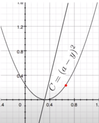
We can find how it will change with respect to the activation: (This is just for the activation, we will differentiate it wrt to the weights when we get to the chain rule.)

$$\frac{\partial C}{\partial a}=2(a-y)$$

This will tell us how fast, or which direction will decrease the cost most quickly. So when we change the weights, we can make the change in the direction of steepest descent. I.e. the ”Gradient” of ”Stochastic Gradient Descent”.

I hear you asking, “if the derivative gives us the shape, why can’t we just immediately pick the point of lowest cost?” Now, this plot is just for only variables (it kinda ignores the a value), in reality the shape is made of combined curves of the many activation functions of all the neurons in the network and each of their unique weights, not to mention it is “changing” between learning steps. While this is a hyperdimensional space (N-dimensional depending on the number of weights in your network), we often illustrate this with a three-dimensional drawing for simplicity (borrowing from 3B1B):

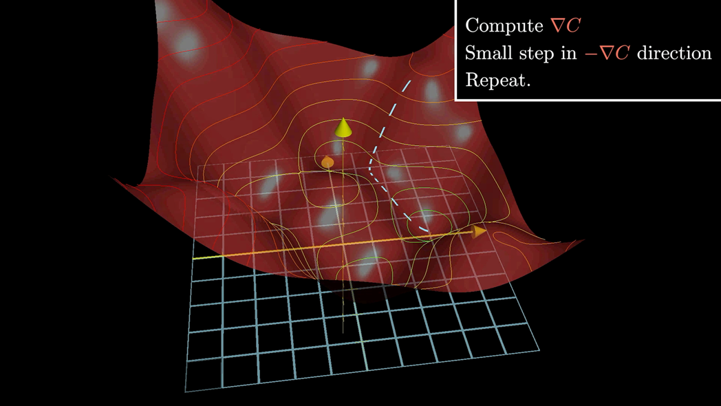
This combination of the curves of the functions gives us the “shape” of the space, which is called the Loss Landscape. Note how he is describing the change in cost as $\nabla C$, but we will get to that when we describe Stochastic Gradient Descent.

Chain Rule

A moment ago we described the the differentiation of the cost wrt to the activation of the last layer, and we will need that so hold on to that, but we want to differentiate the cost, with respect to the weight:

$$\frac{\partial C}{\partial w^{(L)}}$$

I.e. see how the cost changes, so we can move towards setting weights to result in the lowest cost

• However, we need to first differentiate with respect to the activation
• This is because the activation will different at each layer
• And to assign credit properly we will need to chain together the dependencies of activation

This is done with the chain rule:

$$\frac{\partial C}{\partial w_{jk}^{(L)}}=\frac{\partial g_k^{(L)}}{\partial w_{jk}^{(L)}}\frac{\partial a_k^{(L)}}{\partial g_k^{(L)}}\frac{\partial C}{\partial a_k^{(L)}}$$

Ok I’m going to make that easier to look at:

$$\frac{\partial C}{\partial w}=\frac{\partial g}{\partial w}\frac{\partial a}{\partial g}\frac{\partial C}{\partial a}$$

Just remember we are using this is not the correct way to show this, and we are just trying to describe the only weight at the last layer of our simple chain network. The above is more generalized to all possible nodes in all possible layers.

We can further simplify this because the activation function ($g$) we are using is a ReLU, thus

$$g_k=a_j\cdot w_{jk}$$

So we can directly describe our cost in terms of the weights:

$$\frac{\partial C}{\partial w}=\frac{\partial a}{\partial w}\frac{\partial C}{\partial a}$$

• So we differentiate our cost wrt activation

$$C=(a_k-y{)}^2\to \frac{\partial C}{\partial a_k}=2(a_k-y)$$

• And the activation wrt the weight

$$a_k=a_j\cdot w^{(L)}\to \frac{\partial a_k}{\partial w^{(L)}}=a_j$$

• So altogether:

$$\frac{\partial C}{\partial w}=\frac{\partial a}{\partial w}\frac{\partial C}{\partial a}=a_j\cdot 2(a_k-y)$$

Insert the dependency on the weight:

$$\frac{\partial C}{\partial w_{jk}}=a_j\cdot 2((a_j\cdot w_{jk})-y)=2w_{jk}-2$$

Thus, the Cost dependency on $w_{jk}$ is the above. When we want to change to a new weight, we can use the update rule: Where $r$ is a learning rule (we use $r=0.1$)

$$w_{new}=w_{old}-r\frac{\partial C}{\partial w}=w_{old}-0.1\cdot \left(2w_{old}-2\right)$$

This has only been done for a single sample, and thus doesn’t gives us too much information for a single learning step. Thus instead, in actual training, we use batches of input samples and take the average over their output costs. Also important to note here that the $a_j$ is the input value,

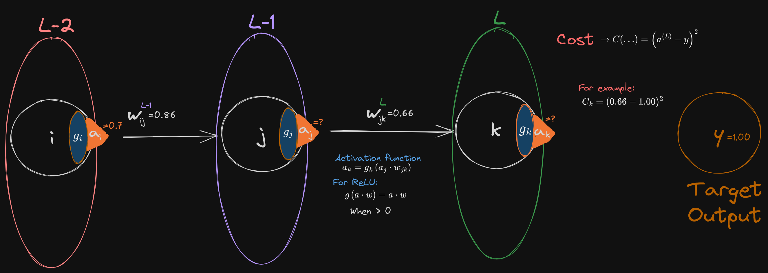
Exercise 1 - Simple Chain Network

Calculate the feed forward for this network, I changed the weights from the original example and illustration so it will be different from before. Then differentiate for $w_{ij}^{L-1}$ and calculate the next weights for the network. You are given: $a_j=0.5$ (the input weight) $w_{jk}^L=0.48$ $y=1.00$ (the target output)

---

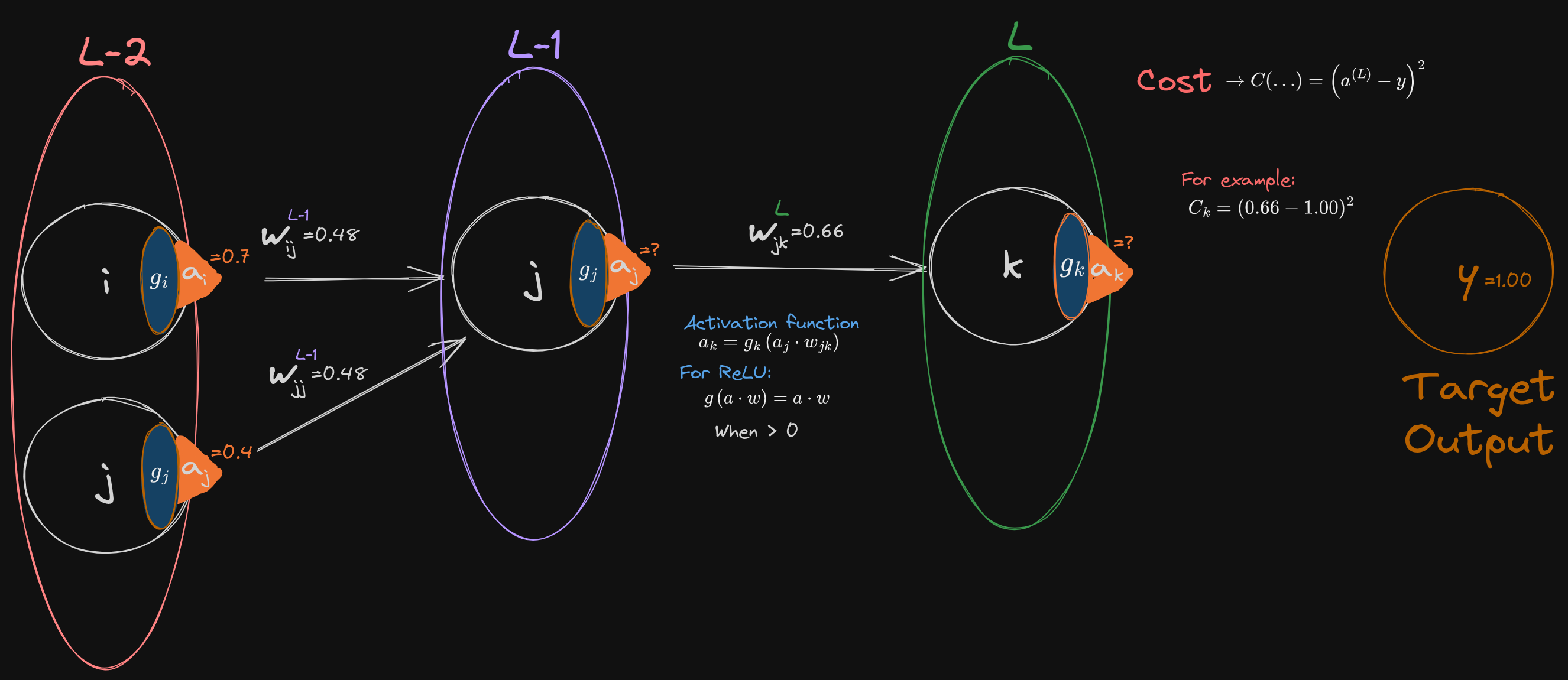
Chain Rule - Deep Chain Network

Ok so I’m going to let you try this one. This one is a little different but not by that much. The difference here is you actually have a hidden layer and $L-2$ is the input layer. In accordance with the chain rule, you can find the derivative but chaining the dependencies of the layers nearest the output. Thus for $w_{ij}^{L-1}$:

$$\frac{\partial C}{\partial w_{ij}^{(L-1)}}=\frac{\partial a_j^{(L-1)}}{\partial w_{ij}^{(L-1)}}\frac{\partial a_k^{(L)}}{\partial a_j^{(L-1)}}\frac{\partial C}{\partial a_k^{(L)}}$$

(I dropped the $g$ again for simplicity, but remember that this won’t be the case for a different activation function) The benefit to this is that you can reuse the derivations that were done for previous layers. You’ve been given the derivation for $\frac{\partial C}{\partial a_k^{(L)}}$ and you even have been given the derivation for $\frac{\partial a_k^{(L)}}{\partial a_j^{(L-1)}}$ if you understand where to plug in what and where (the derivation of a function hasn’t changed, only the variables inserted at the end). You can now reuse that to derive the weight dependency at the last layer. With the chain rule you can do this for as many layers as you need.

Exercise 2 - Three Layer Chain Network

Calculate the feed forward for this network, I changed the weights so it will be different from before. Then differentiate for $w_{ij}^{L-1}$ and calculate the next weights for the network. You are given: $a_i=0.7$ (the input weight) $w_{ij}^{L-1}=0.86$ $w_{jk}^L=0.66$ $y=1.00$ (the target output)

---

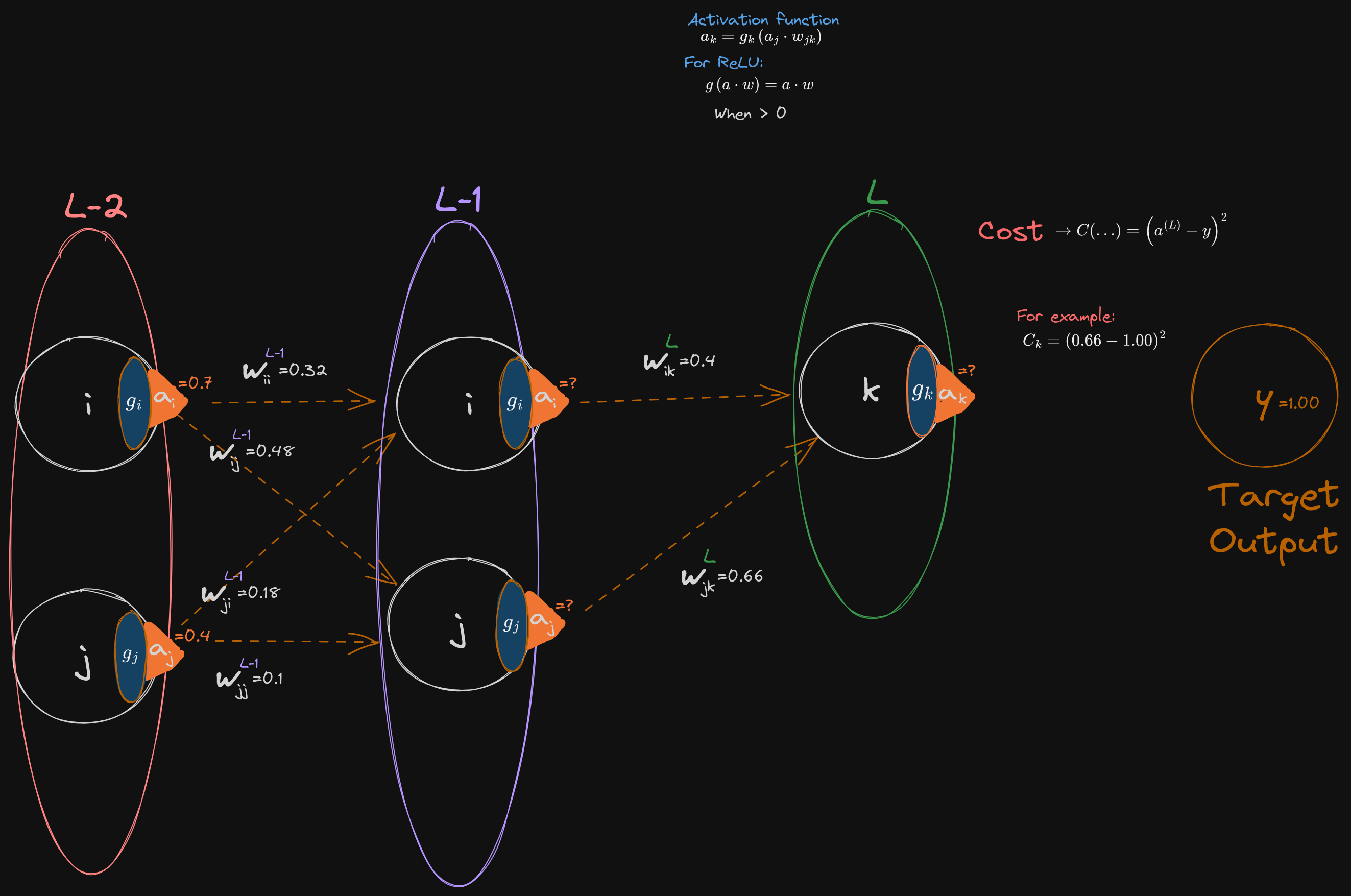
Back-Propagation More Complicated

You can work on this if you’d like some extra practice. And I would actually encourage doing this particular problem.

Note how the unit “numbers” have changed.

• Two input nodes to one Hidden • In_1,2 → Hid → Out

Reminder: $a_j=a_i\cdot w_{ij}^{L-1}+a_j\cdot w_{jj}^{L-1}$

Exercise 3 - Three Layer Chain Network

Calculate the feed forward for this network, I changed the weights so it will be different from before. Then differentiate for $w_{ij}^{L-1}$ and calculate the next weights for the network. You are given: $a_i=0.7$ (the input weight) $a_j=0.4$ (the input weight) $w_{ij}^{L-1}=0.48$ $w_{jj}^{L-1}=0.48$ $w_{jk}^L=0.66$ $y=1.00$ (the target output)

---

Hella Complicated Example

Just re-illustrating the example from the Russell book Chapter 21. Note how the unit “numbers” have changed. Give it a shot if you have literally nothing else to do. There is a reason we make computers do this.