IEEE Neural Engineering 2025

Investigation of Novel SBF-Automata Architecture for Periodicity Finding Solutions at Edge Systems

Download the paper PDF here or continue reading the extended version below.

Presenting at IEEE NER 2025 San Diego, California, USA, 11-14 November 2025

Spotlight Poster Presentation Friday 11:30 - 12:00 || FR2.R3.28

Abstract

Periodicity finding is a critical element in many online learning domains such as web crawling, stock market analysis, robotics, and environmental monitoring. The ability to identify, associate, and internally reproduce intervals of time is a fundamental cognitive element involved in all neural functions in the animal model as well, acting as the basis for learning across the brain. The Striatal Beat Frequency (SBF) model is a well-supported neuroscientific representation of time-intervals within a biological neural architecture and periodicity learning. We transpose the conceptual framework of the SBF into a biologically inspired adaptation, named SBF-Automata (SBF-A): a reinforcement learning (RL) based framework aimed at addressing the periodicity finding problem in real-time and online artificial systems. Initial analysis and simulations indicate that SBF-A provides an attractive alternative to real-time periodicity finding problems at the edge, for which low implementation complexity is of paramount importance.

Introduction

Time-based learning is a critically underdeveloped area in artificial neural networks (ANNs). Moreover, it is virtually absent in online and deep-learning models, which lack the capability to learn temporal associations in real-time edge deployments. Paradoxially, biological neuronal networks are inherently time-based, as evidenced by mechanisms ranging from the firing intervals of spiking communication and spike-timing-dependent plasticity to the larger scale temporal coordination of regional and global brain oscillations Buzsáki et al. (2023). Neural dynamics operate across a wide range of time scales, from milliseconds to the representation of time over seconds, minutes, and beyond Sawatani et al. (2023).

Identifying time intervals between significant temporal points, or detecting the regular or semi-regular occurrence of events over time, constitutes the periodicity finding problem, a common challenge in both natural and artificial systems. In animals, this problem corresponds to Interval Timing (IT): the brain’s capacity to track and associate external events over specific time intervals. Within the field of neuroscientific reinforcement learning (RL), IT is typically studied using the Fixed-Interval (FI) task Swearingen et al. (2010). In this task, a subject is conditioned to learn a specific time interval by associating a stimulus with a rewarded action. Each trial begins with a stimulus, and once the target time interval - referred to as the criterion time $T_C$ - has elapsed, a reward becomes available, contingent on a particular action (e.g. pressing a lever.) For humans, perceivable time intervals generally range from sub-second to supra-second scales ($\sim 300-1000ms$) Petter et al. (2018). Investigating how $\sim 10ms$ neuronal dynamics scale to enable IT could inspire novel and improved designs for ANNs.

Associating events separated in time represents a fundamental challenge for systems operating in dynamic and time-sensitive environments. Periodicity finding problems, such as those encountered in web crawling, online learning, feedback control, and environmental monitoring, depend on the prediction of temporal properties within otherwise noisy data streams. Current approaches to periodicity finding often rely on computationally complex methods, which may be incompatible with the low-energy, real-time processing demands of edge hardware Cooley et al. (1965). Traditional neuroscientific models of IT are influenced by Von Neumann computing paradigm, wherein dedicated neural modules are required for clocking and storing memorized time intervals. However, such models remain poorly defined at the level of neuronal architecture tallotNeuralEncodingTime2020.

The Striatal Beat Frequency (SBF) model is a neuroscientific model of IT and periodic activity reproduction in mammalian brains Matell et al. (2000)Matell et al. (2004), which offers features appealing to machine learning (ML): decentralized &{} asynchronous temporal processing, leveraging of existing neural mechanisms, and integration of activity from assemblies handling other stimulus aspects Buhusi et al. (2005). The SBF model incorporates well-established neural circuits for motor control, execution, reinforcement, and reward, with its neurobiological architecture strongly validated through simulation Allman et al. (2012). The model consists of endogenous oscillators with diverse frequencies, driven by individual neuronal firing rates or population activity. Oscillatory pulses are sent to downstream “coincidence detectors,” which associate these pulses with meaningful stimuli. Upon top-down reinforcement (e.g. a salient event or reward), the phase pattern of synchronized oscillatory activity is encoded in the weights of a neuronal ensemble Gu et al. (2015).

As the SBF model encodes internal time information on the distribution of weights in a minimal neural network, it is an ideal candidate for ANN applications. The biologically inspired method of learning and modifying weights may provide a novel low-complexity and low-energy alternative to traditional methods utilized in deep neural networks. Although SBF is a well-supported neuroscientific model of RL in animal behavior with implementations in simulation Allman et al. (2012), it has not yet been introduced to a ML context.

We propose SBF-Automata (SBF-A) in this work: an adaptation of the SBF model into a RL framework for use in continuous activation ANNs in resource constrained real-time edge applications. As the SBF-A follows a neuronal spiking paradigm, the model is suitable for implementation in ultra-low-power and asynchronous hardware, such as autonomous robotics and edge computing devices deployed in resource constrained environments Zhang et al. (2023)Reza (2022).

Unlike traditional RL models which rely on tabular data storage, The SBF-A encodes learned policies directly into the weights of the network. This differs from Deep-RL methods Mnih et al. (2015), as Deep-RL networks are incapable of online learning, and rely on large sample batches over multiple epochs. Unlike back-propagation, SBF-A applies weight updates locally, allowing for online, in-situ, and few-shot learning. The original contributions of the work can be summarized as follows:

1. the SBF-A: a novel automata model with oscillator and executive units with potential scalability to large networks
2. a family of weight update algorithms for the SBF-A, capable of learning and reproducing periodic activity
3. comparison of the computational complexity, learning performance and accuracy of the SBF-A model against standard periodicity finding approaches,
4. comparison across alternative SBF-A weight distribution algorithms using metrics that provide insights into differences in delay, accuracy, activity and energy consumption.

In the following section, we outline how the basis of the SBF model can be fitted to a learning automata context in a novel neural model of learning: the SBF-A. We establish the general framework of the SBF-A, as well as the family of weight update algorithms that have been successfully deployed. In sections computational complexity and methods we draw comparisons between the SBF-A and established periodicity finding methods, and outline the experiments applied to evaluate the SBF-A model, respectively. The results and discussion section are followed by conclusions from this work.

SBF-A

SBF-A is a naive RL model based on SBF with two main parts: 1. the oscillator block, containing a set of oscillator units, each of which ”peaks” in activity at a unique periodicity; and 2. the executive unit, which integrates the individual unit activity from the oscillator block and decides whether or not to perform an action.

Oscillator units act discretely, mimicking the tonic firing of a single neuron. An individual unit has a unique periodicity $\theta$ i.e. it activates on time-steps coinciding with its period. For example, unit $i$ with ${\theta }_i=3$ has activity $a_i=1$ during time-step $t=3,6,9,\dots$ (Illustration 1). Each oscillator is weighted. Initial weights are evenly distributed, such that initial weights are $w_i=1/N_{osc}$, where $N_{osc}$ is the total number of oscillator units in the set. A special oscillator with zero-periodicity, termed the no-action oscillator, is also included in this set. This unit votes for no-action at every time-step, acting as a broad inhibitory signal, tempering hyperactivity by absorbing excess weight in the system.

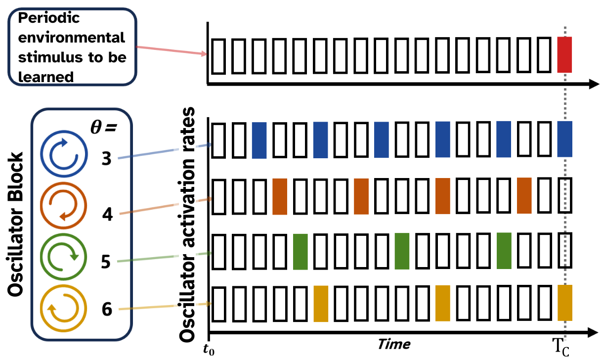Illustration 1: Depiction of discrete oscillator unit activity corresponding to the time-space

At the start of a new trial all oscillator phases are reset to their initial state. Oscillators then run continuously until a reset signal is received, denoting the start of a new trial. At each time-step $t$, activity from oscillator units whose periods exactly divide the current time-step is projected to the executive unit. The executive unit then makes a Markov decision based on the weighted and summed activity. If an action is taken by the SBF-A, the environment then elicits a response (reward, no-reward) conditional on if the action has been performed on a valid time-step. Upon receiving environmental stimulus, the SBF-A updates its weights and learning parameters according to the chosen algorithm, taking into account the reward signal received from the environment $r(t)=[0,1]$. After some period of training, the distribution of weight should correspond to a distribution of oscillatory signals which best inform the executive unit to act on the correct time-steps.

E.g.: when an action is taken at the correct time, a feedback signal from the environment triggers a “reward” update, strengthening or weakening weights corresponding to the activity contribution of the oscillator units. Reversely, a “punishment” update may be performed when the executive unit takes action on an incorrect time-step.

Model Initialization

Each oscillator $i$ is assigned a unique periodicity ${\theta }_i$, selected from a uniformly distributed range to ensure diverse activation patterns. Initial weights $w_i(0)$ are assigned uniformly across all oscillators:

$$\begin{array}{r}\begin{array}{r}{w}_i(0)=\frac{1}{N_{\text{osc}}}\end{array}\end{array}.$$

These weights are normalized such that the total weight across all oscillators sums to one.

Operational Stages

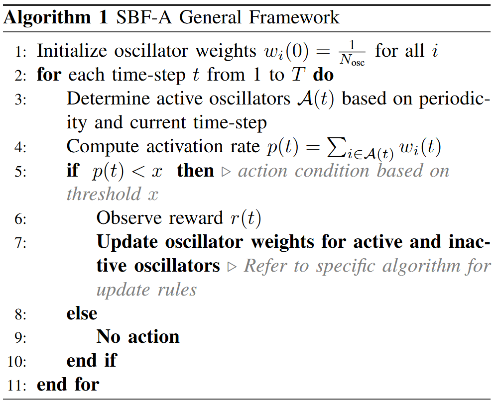
The SBF-Automata operates in two distinct phases at each time-step: Activiation Stage:

• Determine the set of active oscillators $\mathcal{A}(t)$, where $\mathcal{A}(t)=\{i:a_i(t)=1\}$. - An oscillator unit is defined as active if its cyclic period is in phase with the current time-step. If $tmod{\theta }_i=0$ then $a_i(t)=1$, else $a_i(t)=0$.
• Calculate the activation rate $p(t)$ as the sum of weights of active oscillators: $p(t)={\sum }_{i\in \mathcal{A}(t)}{w}_i(t)$.
• Assess whether action occurs by comparing $p(t)$ against a random number $x$ uniformly distributed between zero to one: $\{x\in \mathbb{R}\mid 0\le x\le 1\}$, such that probability of action corresponds to $p(t)$.

Selection Stage:

• If action occurs ($p(t)\ge x$):
  • Observe the reward signal $r(t)$. - Apply weight update rules for active and inactive oscillators based on the observed reward.|
• If action does not occur ($p(t)<x$):
  • No action is taken; weights remain unchanged.

The reader may refer to Algo. 1 – SBFA for algorithmic format.

Algorithm 1 – SBF-A General Framework

Algorithms

Four different SBF-A algorithms are investigated as part of this work, each differ in how oscillator weights are redistributed based on state-action-reward feedback. The choice of algorithm depends on the desired sensitivity to reward magnitude and the specific learning dynamics required for the chosen task. The general weight update procedure is outlined next, followed by details of different algorithms.

Key Components and Definitions

• $N_{\text{oscillators}}$: Total number of oscillators.
• ${\theta }_i$: The assigned cyclic activity period for oscillator $i$
• $a_i(t)$: Activation of oscillator unit $i$ at time-step $t$ (1 if active, 0 otherwise)
• $w_i(t)$: Weight of oscillator unit $i$ at time-step $t$. $w_i=[0,1]$
• $r(t)$: Reward signal at time-step $t$
• $\lambda$: Learning rate parameter
• $\beta$: Penalty parameter
• $\alpha$: Reward learning parameter
• $W_{\text{active}}(t)$: Total weight of active oscillators at time-step $t$
• $W_{\text{inactive}}(t)$: Total weight of inactive oscillators at time-step $t$
• $N_{\text{active}}(t)$: Number of active oscillators at time-step $t$
• $N_{\text{inactive}}(t)$: Number of inactive oscillators at time-step $t$
• $c_i(t)$: Proportional contribution of oscillator $i$ at time-step $t$
• $T_C$: The criterion time, i.e. target time period at which reward is available

SBF-A General Update Procedure

Identify Active and Inactive Oscillators:

• Based on the current time-step and each oscillator’s periodicity. Compute Activation Metrics:
• $W_{\text{active}}(t)$: Total weight of active oscillators at time-step $t$
• $W_{\text{inactive}}(t)$: Total weight of inactive oscillators at time-step $t$
• $N_{\text{active}}(t)$: Number of active oscillators at time-step $t$
• $N_{\text{inactive}}(t)$: Number of inactive oscillators at time-step $t$
• Total weight of active oscillators at time-step $W_{\text{active}}(t)$,
• $W_{\text{inactive}}(t)$,
• $N_{\text{active}}(t)$,
• $N_{\text{inactive}}(t)$. Apply Update Rules:
• Depending on the observed reward $r(t)$ and the specific algorithm, adjust the weights $W_i(t)$ accordingly.

Uniform Redistribution - Magnitude Agnostic (UR-MA)

The Weighted Majority Algorithm (WMA) Littlestone et al. (1994) is the basis for the UR-MA weight redistribution algorithm. The algorithm is Magnitude Agnostic (MA) in that the environmental reward is interpreted as a boolean, ignoring any reward value magnitude. In any reward-state the weight is redistributed from oscillator units which are in “incorrect” state, i.e. when no reward is retrieved, weight is redistributed from active units to inactive units, and when reward is retrieved, weight is redistributed from inactive units to active units. We uniformly apply this redistribution by summing the weights of units in the incorrect state, adjusting the amount scaled by the learning parameters ($\alpha ,\beta$), and evenly applying the sum of that weight to units in the “correct” state, while reductively scaling the “incorrect” unit weight. The UR-MA is given by: Reward ($r(t)>0$):

$$\begin{array}{r}{w}_i(t+1)=\{\begin{array}{ll}{w}_i(t)+\frac{W_{\text{inactive}}(t)\cdot \alpha }{N_{\text{active}}(t)},& \text{if active},\\ w_i(t)\cdot (1-\alpha ),& \text{if inactive}.\end{array}\end{array}$$

Punishment ($r(t)=0$):

$$\begin{array}{r}{w}_i(t+1)=\{\begin{array}{ll}{w}_i(t)\cdot (1-\beta ),& \text{if active},\\ w_i(t)+\frac{W_{\text{active}}(t)\cdot \beta }{N_{\text{inactive}}(t)},& \text{if inactive}.\end{array}\end{array}$$

Uniform Redistribution - Magnitude Sensitive (UR-MS)

The UR-MA is extended to the Magnitude Sensitive (MS) variant, the UR-MS. The UR-MS recognizes and integrates the magnitude of the reward signal $r=[0,1]$, eliminating separate handling of reward and punishment cases, and redistributing weight proportionally with actual amount of reward retrieved. This allows the redistribution algorithm to account for how “close” oscillator units were to the target. This is useful in cases where a freshness measure is applied to reward. The UR-MS is given by:

$$\begin{array}{r}{w}_i(t+1)=\{\begin{array}{ll}{w}_i(t)+r(t)\cdot \frac{W_{\text{inactive}}(t)\cdot \alpha }{N_{\text{active}}(t)}& \\ -(1-r(t))\cdot w_i(t)\cdot \beta ,& \text{if active},\\ w_i(t)\cdot (1-r(t)\cdot \alpha )& \\ +(1-r(t))\cdot \frac{W_{\text{active}}(t)\cdot \beta }{N_{\text{inactive}}(t)},& \text{if inactive}.\end{array}\end{array}$$

Proportional Contribution Redistribution (PCR)

Uniform Redistribution algorithm is further enhanced into Proportional Contribution Redistribution (PCR). Taking inspiration from Long Term Potentiation (LTP) learning in the neuronal model Gerstner et al. (2018), the weights are adjusted based on the individual unit contribution relative to the total oscillator activity. Hence, the weight redistribution is scaled proportional to the weighted sum of activity. The PCR formula is:

$$\begin{array}{r}{c}_i(t)=\{\begin{array}{ll}\frac{w_i(t)}{W_{\text{active}}(t)},& \text{if active},\\ & \\ \frac{w_i(t)}{W_{\text{inactive}}(t)},& \text{if inactive},\end{array}\end{array}$$

where $c_i(t)$ is the relative contribution of unit $i$ at time-step $t$. The PCR for the MA regime (PCR-MA) is defined as,

$$\begin{array}{r}{w}_i(t+1)=\{\begin{array}{l}{w}_i(t)+c_i(t)\cdot W_{\text{inactive}}(t)\cdot \alpha ,\\ \text{if }r(t)>0\text{ and active},\\ w_i(t)\cdot (1-\alpha ),\\ \text{if }r(t)>0\text{ and inactive},\\ w_i(t)+c_i(t)\cdot W_{\text{active}}(t)\cdot \beta ,\\ \text{if }r(t)=0\text{ and inactive},\\ w_i(t)\cdot (1-\beta ),\\ \text{if }r(t)=0\text{ and active},\end{array}\end{array}$$

and is expanded to the MS regime (PCR-MS) as,

$$\begin{array}{r}{w}_i(t+1)=\{\begin{array}{l}\begin{array}{rl}{w}_i(t)+r(t)\cdot c_i(t)\cdot W_{\text{inactive}}(t)\cdot \alpha & \\ -(1-r(t))\cdot w_i(t)\cdot \beta ,& \text{if active},\end{array}\\ \begin{array}{rl}& \\ (1-r(t))\cdot c_i(t)\cdot W_{\text{active}}(t)\cdot \beta & \\ +w_i(t)\cdot (1-r(t)\cdot \alpha ),& \text{if inactive}.\end{array}\end{array}\end{array}$$

This brings the algorithm more in-line with a Dopaminergic LTP learning rule Gerstner et al. (2018), where strength of the reward attenuates the learning error during weight updates.

Computational Complexity

Complexity Per Update Step in SBF-A

Unlike traditional time-stepped algorithms, the SBF-A does not necessarily update its weights at every time-step. An update occurs only when the system takes an action. Determining which oscillators are active and redistributing weights both require at most $O(N)$ work, where $N$ is the number of oscillators: Check Active Oscillators: For each oscillator, we verify whether its period divides the current time index. This is a linear pass across $N$ oscillators. Weight Update: Whether we use PCR, or UR rules, each update step loops over the $N$ oscillators to adjust weights. Hence, each update step takes $O(N)$ time, even if multiple oscillators happen to be active at once.

Biological Plausibility of SBF-A

In addition to being computationally light at $O(N)$ per update, SBF-A exhibits several neurophysiological advantages: No Central Clock: By encoding time in a diverse set of oscillators, our method dispenses with centralized timing mechanisms. Local Synaptic-Like Updates: Weight changes reflect simple, localized reward or penalty signals rather than complex global error gradients. Distributed Storage of Time: Each oscillator provides partial information about periodic structure, collectively forming a robust, decentralized representation.

Contextual Bandit Complexity in Comparison

A contextual bandit perspective typically entails more expensive update steps. For example, LinUCB Lattimore (2020) requires inverting (or rank-1 updating) a $N\times N$ matrix, where $N$ is the number of features. Naive inversion costs $O(N^3)$ per update.

Even if updates do not happen every step, any LinUCB update must handle matrix operations of $O(N^3)$ complexity, significantly higher than the $O(N)$ in SBF-A. Moreover, matrix inversion is not obviously analogous to local synaptic changes in a biological neuron population, making the approach less neurophysiologically plausible.

Implications for Scalability and Biological Inspiration

Since each SBF-A update step is $O(N)$, it scales favorably with the number of oscillators. By contrast, LinUCB’s matrix operations inflate to $O(N^3)$ per update step. This divergence becomes critical as $N$ grows. Furthermore, SBF-A’s incremental weight shift reflects the kind of distributed, asynchronous processing observed in real neural circuits. Thus, both from a computational and biological standpoint, SBF-A offers a simpler and more plausible pathway to periodic learning.

Methods

Experimental Task (FI Task)

Interval Timing is considered crucial for causal inference, decision making, and reward value estimation Mello (2016). The common method for testing IT in animal models is the Fixed-Interval (FI) task Swearingen et al. (2010), where an animal is conditioned over repeated trials to infer an interval of time by associating an initial stimulus with a rewarded action. A task trial is initiated by a stimulus. Once the target time interval, the criterion time $T_C$, has elapsed, a reward is available for retrieval through an action, e.g. pressing a lever.

While the animal is free to perform this action at any time during the interval, reward will only be available after the $T_C$ has been reached and for a short time after. It is the animal agent’s prerogative to retrieve the reward as soon as possible. When in an unlearned state, it will follow an exploratory policy by uniformly attempting action over time until the reward is obtained. As the animal learns, its actions converge about the correct time across repeated trials.

In the basic SBF-A verification environment, trial time-space is divided into discrete time-steps: $t=0,\dots ,T_{end}$, over which several FI trials are run.

We replicate the FI as RL task, where the automata is made to learn a target time interval, $T_C$, by associating an initial stimulus with a reward. A the beginning of each experiment, the automata is given a start signal to mark a new trial and the start of the interval to be timed. During the interval, no reward is available, and actions taken by the automata elicit no response until the $T_C$ is reached. Reward is available for some window of time after the $T_C$ before the trial is reset. The first action taken by the automata, at or after the time-step corresponding to the $T_C$, retrieves the reward. The SBF-A resets all oscillators to their initial phase upon obtaining the reward. Likewise, the trial timer resets $t=0$, and a new task trial begins. This is repeated for some number of trials, over which the automata is expected to arrive at an internal approximation solution for the $T_C$.

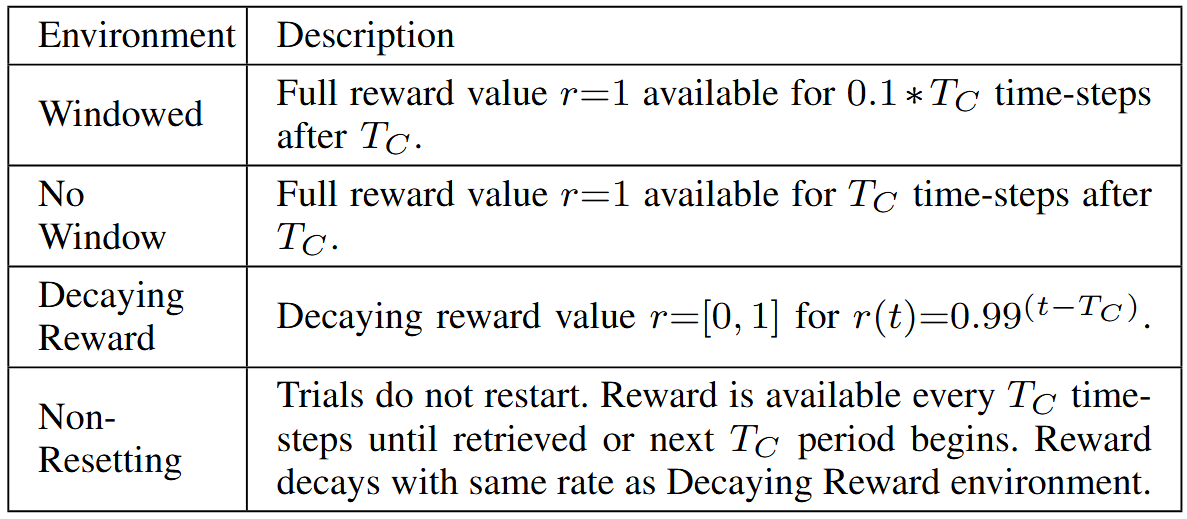
The first environment variant tested is the Windowed environment, where the full reward value $r=1$ is available for $0.1\ast T_C$ time-steps after $T_C$. Following this, a No Window environment is also tested, where there is no limitation to how soon the reward can be retrieved. A freshness measure is added for a Decaying Reward environment, where reward value is proportional to how quickly it is retrieved by the model, with reward at its maximum value of $r=1$ at the $T_C$ and decaying at a log-rate with each subsequent time-step, until retrieved by the automata. Decay rate is scaled to the $T_C$. It is worthwhile to note that decay is ignored in the MA algorithms which interpret any reward as having full value, regardless of the actual value. The last variation is the Non-Resetting environment. In this environment, the reward is available with static periodicity, which does not reset to zero on the start of a new trial, and instead is continuously running. The SBF-A oscillators still reset upon retrieval of reward. Reward value decays and is available until retrieval. This emulates classic periodicity finding problems such as optimal web-crawling Han et al. (2020) and provides a challenge to the model as it can no longer rely on an initializing stimulus. Environment variants in the experimental task are summarized in Table 1 – Environmental Variants.

Table 1 – Environmental Variants

Experimental Regime

Using a toy model as a proof of concept, the SBF-A’s efficacy in identifying and learning a target time interval, is studied. The SBF-A and its update algorithms are capable of converging to the solution $T_C$ when given as a context choice in an oscillator unit’s period: ${\theta }_{solution}=T_C$. The capabilities of the SBF-A in the naive regime, in which no solution oscillators are provided, are examined next. In this regime, learned time-periods must be internally represented in the distribution of weights in the ensemble. It is expected that the discrete SBF-A is limited in performance by the number of oscillator units used. The relatively few oscillator units used in the regime with the largest oscillator set size, $N_{osc}<12,000$ with uniformly distributed periods and rigidly discrete tonic activity, may show less overlap or coordinated activity in comparison to other simulations Allman et al. (2012) which are able to create overlapping receptive fields. Understanding such limitations is an important aspect of the experiment. The relationship between oscillator set density and distribution of oscillator periods with respect to performance, as well as the comparative performance of the update rules are investigated in the naive case. It is expected to observe an increase in model accuracy as oscillator set density (total number of oscillators) increases. All experiments and simulations are carried out in Python; code is available upon request.

The SBF simulation by Allman et al. (2012) uses 15,000 discrete firing neurons, effectively creating a sinusoidal receptive field (the temporal ”field” of coverage by the model) via dense population activity. Oprisan et al. (2022), reduces this to single ”units” with sinusoidal activity of varying periods. The SBF-A falls between the Oprisan sinusoidal model and the Allman and Meck 2012 SBF simulation.

Periodicity Finding Methods Comparison

The SBF-A is compared against several common time-series periodicity finding methods, including the Fast-Fourier Transform (FFT) Cooley et al. (1965), the Auto-Correlation Function (ACF) Broersen (2006), and Autoperiod Vlachos et al. (2005) methods. The above algorithms are tested against the PCR-MS in the toy regime with Decaying Reward and Non-resetting environments. For each trial the PCR-MS activity and reward are recorded as a sparse time-series where: $0$ is no action, $-1$ is miss, and $+1$ is action with reward. At the end of each trial (retrieval of the reward) the resulting time-series is input to the other methods and their resulting period estimate is recorded for that trial. We directly compare the performance of the standard methods against the SBF-A in fig. 2 .

Figure 2 - Comparison of PCR-MS SBF-A against standard periodicity prediction methods.

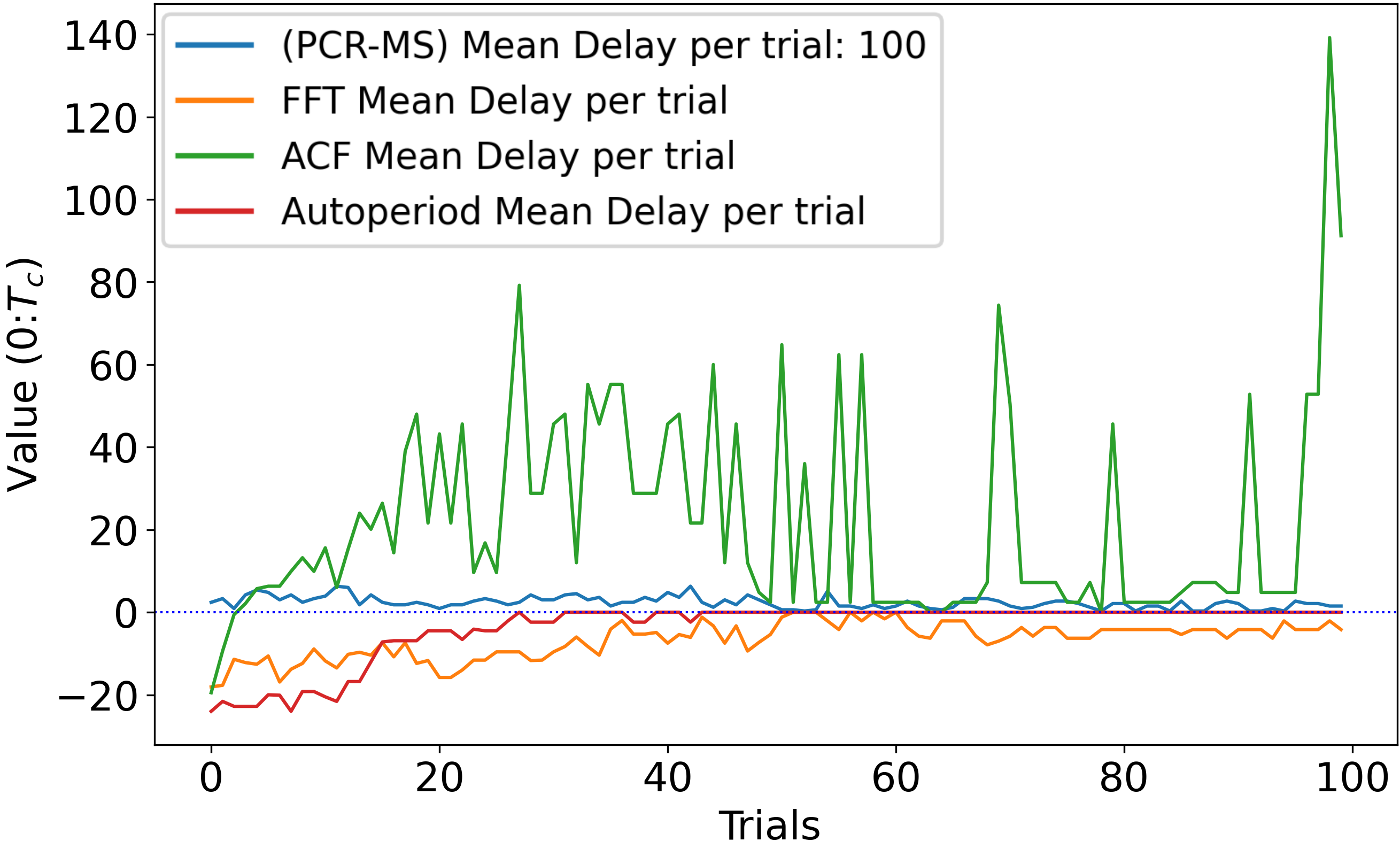Y-axis is the mean delay. X-axis is the trial number in the experiment. Values are averaged over 100 experiments.

Metrics

Metric statistics are averaged over a hundred independent sessions with identical experimental conditions. We measure the SBF-A in accuracy, and efficiency: learning the $T_C$ while reducing the number of actions taken. We define our metrics as follows:

Convergence: The ability to converge to a stable distribution of weights internally representing the solution.

Delay: Time to first correct action after $T_C$ as a measure of accuracy. Lower is better.

Latency: Time to convergence. The earliest trial where peak Delay value is found, measured in time-steps. Lower is better.

Stability: The standard deviation in accuracy (Delay) after Convergence. Lower is better.

Energy: Total actions performed over the lifetime of the model, multiplied by the Latency. Lower is better.

Results

Toy Regime

The toy regime is tested for a $T_C=24$ and a predefined oscillator period distribution set of $\theta =\{3,6,12,24,36,48\}$. This regime does not use a no-action oscillator. The SBF-A algorithms successfully maximize the weight of the correct oscillator unit $\theta =24$. The weights are redistributed so that the oscillator with the same period as the $T_C$ obtains the largest weight, while the weights of oscillators whose periods subdivides the $T_C$ have weights distributed to them proportional to how often they correctly contribute, and inversely proportional to how often they incorrectly contribute.

Evaluation of SBF-A

The decaying reward value can be observed as a metric of how the SBF-A develops in precision over time. In Fig. 1 the value of the reward recovered is plotted alongside the number of actions taken by the automata agent per trial. All values average from one hundred sessions. The SBF-A maintains a high performance, staying over a mean reward value of $R>0.89$ and increasing to $R\sim 0.95$ after convergence. The average number of actions per trial, starts out relatively low, and decreases further over time to reach stability. While the SBF-A solution effectively reaches convergence at trial 60-73 (Table 2), oscillator weights continue to progress and separate until the end of the session.

Fig. 2 illustrates the average delay (total time-steps over the $T_C$ when action is taken) against the periodicity prediction of the other methods. The SBF-A maintains an advantage in stability, speed of learning, and accuracy.

Figure 1 – Mean reward value retrieved and mean actions per trial.

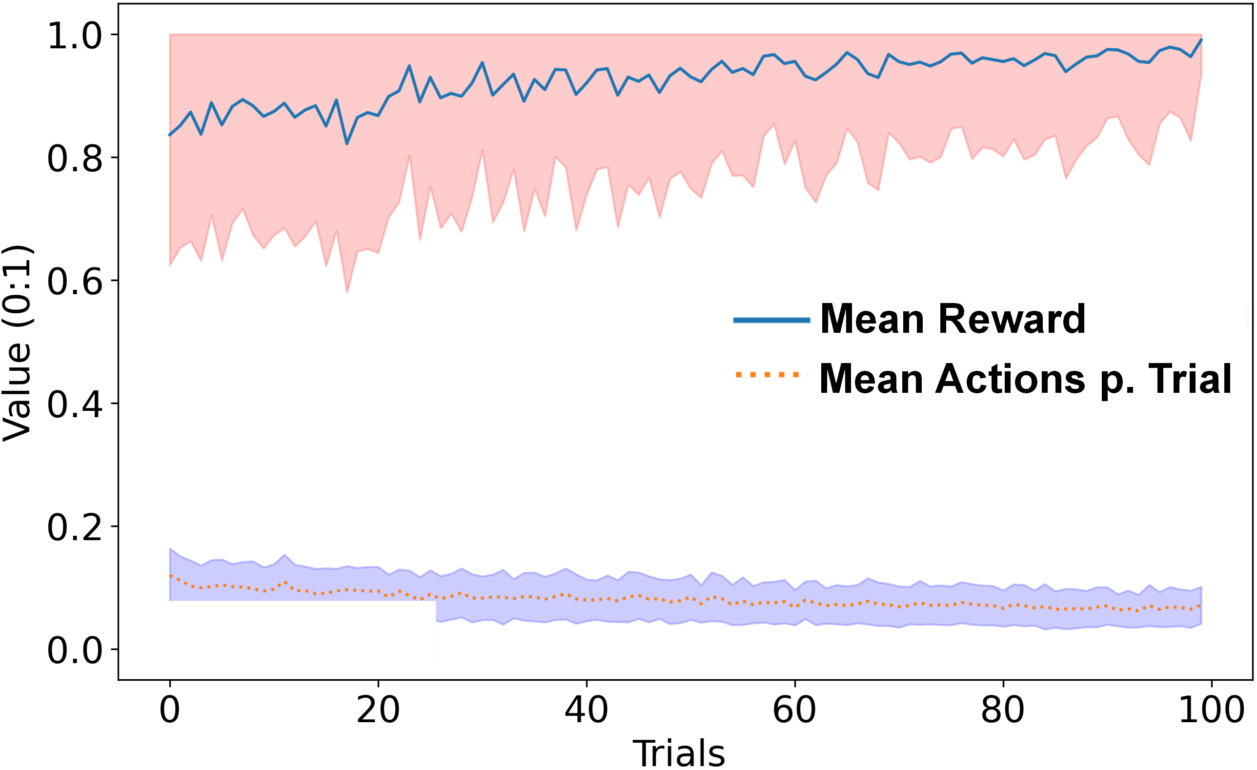Action total is normalized to trial size (TC ). Shaded areas represent the first normal Std Dev.

Table 2 – Toy Model Results

Delay is the Peak Delay value, normalized to $T_C$ . ”STD” is the Delay Standard Deviation normalized to $T_C$. ”Lat.” is Latency. Energy is the total activity of the model multiplied by the normalized Peak Delay value (lower is better).

Comparison of SBF-A Weight Distribution Algorithms

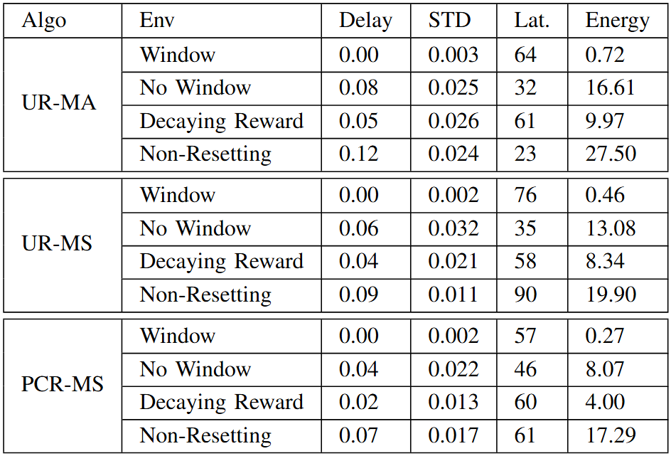
Comparing the performance of different algorithms in Table \ref{tab:table1}, the PCR-MS is the most robust, maintaining the highest accuracy scores in all environments against the UR algorithms. The trade-off is a slight increase in actions taken, however, this is negligible in comparison with only a $\sim 2-4\%$ increase in total activity over the other algorithms.

Naive Regime: Distribution and Density

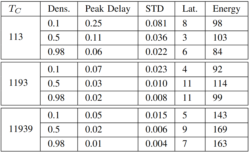
The true measure of the SBF-A’s efficacy, is applying it in a naive regime where a solution is not explicit. Instead, collective oscillator activity is required to compute a solution. PCR-MS is used in this example with a decaying reward environment and three different $T_C$ resolutions: $T_C=\{113,1193,11939\}$ We use prime numbers to avoid the simplicity of sub-divisor oscillator periods. The oscillator periods are uniformly distributed between $\theta =0$ (the no-action oscillator) and a max periodicity of $\theta =0.99\ast T_C$. We avoid a “first-past-the-post” oscillator, to ensure a solution must be more distributed across the weights.

In all $T_C$ regimes, the accuracy improves as the oscillator density (number of oscillators per set respective to size of time interval) increases, which matches predictions based on biological precedence. This can be observed in Table 3. The differing behavior in higher time resolutions is noteworthy, where accuracy increases with resolution alongside oscillator density. This may have something to do with a greater ability for oscillator periodicities to overlap and cover shorter periods. The weight distributes far more diffusely in the denser regimes, and with differing patterns of distribution across the different $T_C$. While the oscillator weights distribute with more variance and chaotic behavior over time, the solution stays stable and converges early.

Table 3 – Naive Regime: PCR-MS Decaying Reward

Delay is the Peak Delay value, normalized to $T_C$ . ”STD” is the Delay Standard Deviation normalized to $T_C$. ”Lat.” is Latency. Energy is the total activity of the model multiplied by the normalized Peak Delay value (lower is better).

Conclusion

We have shown the SBF-A effectively addresses the periodicity finding problem in artificial systems. Our approach offers an efficient solution for identifying temporal patterns without requiring explicit temporal encoding or state comparisons. In our experiments, we demonstrate that the SBF-A successfully converges under multiple temporal regimes for the FI task, while also maintaining a high degree of computational efficiency and accuracy, supporting its potential applicability for temporally based RL tasks in dynamic real-world domains with extreme energy constraints. This opens the SBF-A framework to future exploration in more challenging and complex scenarios.