PENG9570 — Lecture 8

Uniqueness theorem for solution of the 1D heat / diffusion IBVP

The IBVP:

$$\begin{array}{rl}& u_t=k{u}_{xx},0<x<l,t>0.\\ & u(0,t)=g(t),0<t<T\\ & u(l,t)=h(t),0<t<T\\ & u(x,0)=f(x),0<x<l\end{array}$$

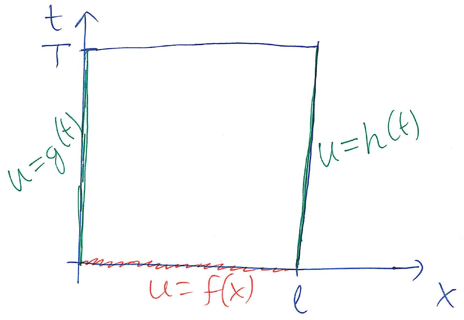
Theorem:

The solution $u(x,t)$ of the IBVP is unique.

Proof:

We assume that there are two solutions $u$ and $v$. Set $w=u-v$. Then:

$$\begin{array}{rl}{w}_t-k{w}_{xx}& =u_t-v_t-k\left(u_{xx}-v_{xx}\right)\\ & =\underset{=0}{\underbrace{\left(u_t-k{u}_{xx}\right)}}-\underset{=0}{\underbrace{\left(v_t-k{v}_{xx}\right)}}\\ & =0-0=0\end{array}$$

So, $w$ is a solution of $w_t=k{w}_{xx}$, $w(x,0)=u(x,0)-v(x,0)=f(x)-f(x)=0$ $w(0,t)=u(0,t)-v(0,t)=g(t)-g(t)=0$ $w(l,t)=u(l,t)-v(l,t)=h(t)-h(t)=0$

This shows that $\{\begin{array}{ll}{w}_t=k{w}_{xx}& 0<x<l,t>0\\ w(x,0)=0& 0<x<l\\ w(0,t)=w(l,t)=0,& t>0.\end{array}$ We want to show that $w\equiv 0$ : We introduce the “energy integral”:

$$\begin{array}{rl}& E(t)={\int }_0^l{w}^2(x,t)dx\\ & E^{\prime }(t)={\int }_0^l\frac{d}{dt}\left(w^2(x,t)\right)dx\\ & ={\int }_0^{l}2w\cdot \frac{\partial w}{\partial t}dx\end{array}$$ $$\begin{array}{rl}& =2{\int }_0^{l}w\cdot \underset{=k{w}_{xx}}{\underbrace{w_t}}dx\\ & =2k{\int }_0^{l}w\cdot w_{xx}dx\end{array}$$

Integration by parts:

$$\begin{array}{rl}& \int u{v}^{\prime }dx=uv-\int u^{\prime }vdx\\ & \int w\cdot \underset{\left(w_x\right)x}{\underbrace{w_{xx}}}dx=w\cdot w_x-\int w_x\cdot w_{x}dx\\ & =2k(\underbrace{{\left[w\cdot w_x\right]}_0^l}-{\int }_0^l{\left(w_x\right)}^{2}dx)\\ & w(l,t)\cdot w_x(l,t)-w(0,t)-w_x(0,t)\end{array}$$ $$\begin{array}{rl}& =2k\left(0-{\int }_0^l{\left(w_x\right)}^{2}dx\right)\\ & =-2k\underset{⩾0}{\underbrace{{\int }_0^l\underset{⩾0}{\underbrace{{\left(w_x\right)}^2}}dx}}⩽0\end{array}$$

$E^{\prime }(t)⩽0$; non-increasing $E(t)⩾0$ : non-negative $E(0)={\int }_0^l{w}^2(x,0)dx=0$ Conclusion: $E(t)=0,t⩾0$.

That is,

$$\begin{array}{rl}& {\int }_0^l{w}^2(x,t)dx=0\\ \Rightarrow & w\equiv 0!\\ & u-v=0\\ \iff & u=v\end{array}$$

Only one solution. Uniqueness!

Existence and uniqueness of solution of the IVP $y^{\prime }=f(y),y\left(t_0\right)=y_0$.

The Picard iteration

Integral form of the IVP:

$$y(t)=y\left(t_0\right)+{\int }_0^{t}f(y(s))ds$$

Note: If $u_0(t)\in C[E]$, then all successive elements $\left(u_1(t),u_2(t),\dots \right)$ are also in $C[E]$.

Example:

IVP: $y^{\prime }=y,y(0)=1$. [Exact solution: $y=e^t$]. Solve the IVP using the Picard iteration.

$$\begin{array}{rl}{u}_0(t)& =1\\ u_1(t)& =y_0+{\int }_0^{t}f\left(u_0(s)\right)ds\\ & =1+{\int }_0^t\underset{=1}{\underbrace{u_0(s)}}ds\\ & =1+{\int }_0^{t}1ds=\underline{1+t}\\ u_2(t)& =y_0+{\int }_0^{t}f\left(u_1(s)\right)ds\\ & =1+{\int }_0^t{u}_1(s)ds\\ & =1+{\int }_0^t(1+s)ds\\ & =1+{\left[\frac{1}{2}(1+s{)}^2\right]}_0^t\end{array}$$ $$\begin{array}{rl}& =1+\frac{1}{2}\left((1+t{)}^2-(1+0{)}^2\right)\\ & =1+\frac{1}{2}\left(1+2t+t^2-1\right)\\ & =1+t+\frac{1}{2}{t}^2\\ & u_3(t)=\cdots =1+t+\frac{1}{2}{t}^2+\frac{1}{6}{t}^3\end{array}$$

Sequence of functions are Taylor polynomials of $e^t$ :

$$\underset{n\to \infty }{\lim }{u}_n(t)=e^t$$

Theorem (existence and uniqueness of solution of IVP $y^{\prime }=f(y),y\left(t_0\right)=y_0)$

Let $E\subset {\mathbb{R}}^n$ be open. Assume that $y_0\in E$ and that $f\in C^1[E]$. Then there exists $a>0$ such that the IVP has a solution $y(t)$ on $[-a,a]$ (existence). This solution is unique.

Demonstration of lack of uniqueness Consider the IVP

$$y^{\prime }=\sqrt{y},y(0)=0$$

$y_1\equiv 0$ is one solution. $y_2=\frac{1}{4}{t}^2$ is another solution. $\left[y_2^{\prime }=\frac{1}{4}\cdot 2t=\frac{1}{2}t,\sqrt{y_2}=\frac{1}{2}t\right]$ Note: $f(y)=\sqrt{y}\Rightarrow f^{\prime }(y)=\frac{1}{2\sqrt{y}}$ $f\notin C^1[E]$, $0\in E$.

Cauchy sequences

A sequence where the elements come arbitrarily close to each other when sequence numbers are sufficiently large: For any $\epsilon >0$ there exists an integer $N$ such that for all $m,n⩾N$

$$\left|x_m-x_n\right|<\epsilon .$$

Completeness

A set $S$ is complete when all Cauchy sequences of elements in $S$ converge to an element in $S$.

Example:

$$\begin{array}{rl}& x_n=\frac{1}{n}\in [0,1].\\ & \underset{n\to \infty }{\lim }{x}_n=0\in [0,1].\end{array}$$

(Complete.) Having established that a sequence in a complete set $S$ is Cauchy, we can conclude that the sequence converges to a limit in $S$.

Sketch of proof:

• Define sequence of approximations using the Picard iteration
• Show that this sequence is Cauchy
• Conclude that the sequence converges to an element in $C[E]$.
• This proves existence.
• Assume two different solutions
• Show that gives a contradiction
• This proves uniqueness.

Proof of existence:

The sequence ${\left\{u_k\right\}}_k$ is defined by

$$\begin{array}{rl}& u_0(t)=y_0\\ & u_{k+1}(t)=y_0+{\int }_0^{t}f\left(u_k(s)\right)ds\end{array}$$

Showing that $\left\{u_k\right\}$ is Cauchy: For $m>k⩾N$, we have

$$\begin{array}{rl}& |\begin{array}{l}\left|u_m-u_k\right|=\\ +\cdots +u_m-u_{m-1}+u_{m-1}-\\ +u_{k+1}+u_{k+1}-u_k\mid \\ =\mid \left(u_m-u_{m-1}\right)\end{array}+\left(u_{m-1}-u_{m-2}\right)+\\ & +\left|u_{k+1}-u_k\right|\mid \\ & ⩽\left|u_m-u_{m-1}\right|+\left|u_{m-1}-u_{m-2}\right|\\ & +\cdots +\left|u_{k+1}-u_k\right|\\ & ⩽\cdots +\left|u_{m-}-u_{m-1}\right|+\cdots +\left|u_{k+1}-u_k\right|\end{array}$$

(intinitely many differences)

For each of these differences,

$$\begin{array}{rl}& \left|u_{j+1}-u_j\right|\\ =& \mid y_e+{\int }_0^{t}f\left(u_j(s)\right)ds-\left(y_0+{\int }_0^{t}f\left(u_{j-1}(s)\right)ds\right)\\ =& \left|{\int }_0^t\left(f\left(u_j(s)\right)-f\left(u_{j-1}(s)\right)\right)ds\right|\\ ⩽& {\int }_0^t\underset{⩽k|u_j-u_{j-1}|}{\underbrace{\mid f\left(u_j\right)-f\left(u_{j-1}\right)}}\mid ds\end{array}$$

(Lipschitz: $f$ differentiable) $⩽K{\int }_0^t\left|u_j-u_{j-1}\right|ds$

$$\begin{array}{rl}& ⩽[0,k]c[-a,a]\\ & ⩽K{\int }_0^a\left|u_j-u_{j-1}\right|ds\\ & ⩽\underset{t\in [-a,a]}{\max }\left|u_j-u_{j-1}\right|\cdot a\\ & =Ka\cdot \underset{t\in [-a,a)}{\max }\left|u_j-u_{j-1}\right|\end{array}$$

By induction we can prove that

$$\left|u_{j+1}-u_j\right|⩽{\left(k_a\right)}^{j}b$$

where

$$b=\underset{t\in [-a,a)}{\max }\left|u_1-u_0\right|$$

Essential: $Ka<1$ (by choice of $a$).

Going back to |um-uk|:

$$\begin{array}{rl}& \left|u_m-u_k\right|\\ & ⩽\cdots +\underset{⩽{\left(k_a\right)}^{k}b}{\underbrace{u_{k+1}-u_k}}\mid \\ & ⩽\cdots +{\left(k_a\right)}^{k+1}b+{\left(k_a\right)}^{k}b\\ & ={\left(k_a\right)}^{k}b[\underset{\text{Infinite grom. series }}{\underbrace{1+{\left(k_a\right)}^1+{\left(k_a\right)}^2+\cdots ]}}\\ & ={\left(k_a\right)}^{k}b\frac{1}{1-k_a}\underset{k\to \infty }{\overset{1-0}{\to }}\end{array}$$

This proves that

$${\left\{u_k\right\}}_k$$

is a Cauchy sequence. We have $u_k\in C[E]$. $C[E]$ is complete (known). Conclusion: The sequence converges to a limit $u(t):{\lim }_{k\to \infty }{u}_k(t)=u(t)$, where

$$u(t)\in C[E].$$

This proves existence of a solution.

Uniqueness of the solution of the IVP

Assume (for later contradiction) that there are two distinct solutions $u$ and $v$. Further, assume that $|u-v|$ achieves its maximum value at $t_1\in [-a,a]$. Then:

$$\Vert u\Vert =\underset{t\in E}{\max }\mid u\Vert$$ $$\begin{array}{rl}& \Vert u-v\Vert =\left|u\left(t_1\right)-v\left(t_1\right)\right|\\ & =\mid y_e+{\int }_0^{t_1}f(u(s))ds-y_e-{\int }_0^{t_1}f(vs)ds\\ & =\left|{\int }_0^{t_1}(f(u(s))-f(v(s)))ds\right|\\ & ⩽{\int }_0^{t_1}|f(u(s))-f(v(s))|ds\\ & ⩽{\int }_0^{t_1}K|u(s)-v(s)|ds\\ & \begin{array}{l}{f}_{\text{is }}\\ \text{ differentiable }\\ \text{ Lipscritz }\end{array}\begin{array}{r}|f|f\text{ is "Lipschitz", }\\ \text{ then }|f(u)-f(v)|\\ ⩽K|u-v|\end{array}\end{array}$$

$⩽k\cdot \underset{\Vert u-v\Vert }{\underbrace{[(-a,a)]}}\underset{t_1\le a:}{\underbrace{{\int }_0^{t_1}ds}}$ $⩽k\cdot \Vert u-v\Vert \cdot a\begin{array}{rl}& ⩽{\int }_0^{a}1ds\\ & =a\end{array}$ $=Ka\Vert u-v\Vert$ $[$ a was selected such that Kar1] r $1\cdot \Vert u-v\Vert =\Vert u-v\Vert$ $ka<1$ That is, $\Vert u-v\Vert <\Vert u-v\Vert$. Contradiction ⇒ $U=V$ Uniqueness!