PENG9570 Lecture 6

PENG9570 — Lecture 6 (March 11th)

$$\begin{array}{rl}& \frac{-{\hslash }^2}{2m}{\nabla }^2\Psi (\mathrm{r})+V(r)\Psi (\mathrm{r})=E\Psi (\mathrm{r})\\ & \text{ Kinetic }\\ & \text{ Energy }+\begin{array}{l}\text{ Potential }\\ \text{ Energy }\end{array}=\begin{array}{l}\text{ Total }\\ \text{ Energy }\end{array}\end{array}$$ $$\frac{{\partial }^{2}p}{\partial x^2}-\frac{1}{c^2}\frac{{\partial }^{2}p}{\partial t^2}=0,$$

Wave equation for sound

$$\frac{\partial u}{\partial t}=k\frac{{\partial }^{2}u}{\partial x^2}$$

Heat/diffusion equation

equations

$\frac{1}{r_l}\frac{{\partial }^{2}V}{\partial x^2}=c_m\frac{\partial V}{\partial t}+\frac{V}{r_m}$ Cable equation $u_t=u_{xx}+f(u,v)$,

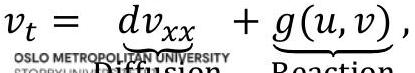Reaction-diffusion equations

Navier-Stokes equations

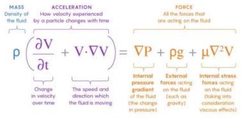
Navier-Stokes Equations Describe the flow of incompressible fluids.

Maxwell’s equations

$\nabla \cdot \mathbf{D}=\rho$	(1)	Gauss’ Law
$\nabla \cdot \mathbf{B}=0$	(2)	Gauss’ Law for magnetism
$\nabla \times \mathbf{E}=-\frac{\partial \mathbf{B}}{\partial t}$	(3)	Faraday’s Law
$\nabla \times \mathbf{H}=\frac{\partial \mathbf{D}}{\partial t}+\mathbf{J}$	(4)	Ampère-Maxwell Law

Partial differential equations (PDEs)

Solution is a function of more than one variable, e.g. $u=u(x,t)$ Examples:

$$\begin{array}{c}{u}_t=k{u}_{xx}+f(u,x,t),\\ u_{xt}=xt\\ \Delta u=f(x,y)\left(\Delta u=u_{xx}+u_{yy}\right)\\ u_x+a{u}_t=0\end{array}$$

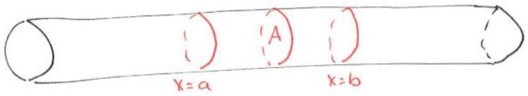
Conservation laws

$u(x,t)$ :Density of a substance Conservation law in differential form:

$$u_t+J_x=f(x,t,u)$$

$J(x)$ : flux of substance (or heat flux) $f(t,x,u)$ : production

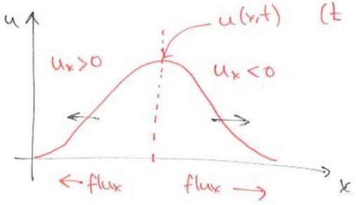
Diffusion (and heat): $J=-D{u}_x\Rightarrow J_x=-D{u}_{xx}$. Then

$$u_t=D{u}_{xx}+f(x,t,u)$$

The heat PDE / Diffusion PDE is a linear PDE

1 D heat PDE / diffusion PDE with source:

$$u_t=k{u}_{xx}+f(x,t),t>0,0<x<L$$

Can be written in terms of the operator $L$ :

$$Lu=f(x,t),Lu=u_t-k{u}_{xx}$$

$L$ is linear since

1. $L(u+v)=L(u)+L(v)$
2. $L(cu)=cL(u)$

For homogeneous problems $Lu=0$, superpositions of solutions are also solutions:

1. $w=c_1{u}_1+c_2{u}_2+\cdots +c_n{u}_n+\cdots$
2. $w={\int }_{I}c(\xi )u(x,t,\xi )d\xi$

Initial boundary value problem (IBVP)

1D heat PDE / diffusion PDE with initial and boundary conditions

$$\begin{array}{cc}{u}_t=k{u}_{xx},t>0,& 0<x<L\\ u(0,t)=a(t),& t\ge 0\\ u(L,t)=b(t),& t\ge 0\\ u(x,0)=g(x),& 0\le x\le L\end{array}$$

Solution is unique (this can be proven) !

Finite difference method for diffusion equation

Consider the 1D diffusion PDE with initial and boundary conditions

$$\begin{array}{c}{u}_t=u_{xx}\\ u(0,t)=u(1,t)=0\\ u(x,0)=g(x)\end{array}$$

Use the approximations

$$\begin{array}{c}{u}_{xx}\approx \frac{u(x+\Delta x,t)-2u(x,t)+u(x-\Delta x,t)}{\Delta x^2}\\ u_t\approx \frac{u(x,t+\Delta t)-u(x,t)}{\Delta t}\end{array}$$

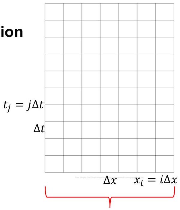
Finite difference method for 1D diffusion equation: grid and explicit scheme

Let $v_{i,j}\approx u\left(x_i,t_j\right)$. Then,

$$\begin{array}{rl}& n+1=7\text{ subintervals. }\\ & \Delta x=1/(n+1)\end{array}$$

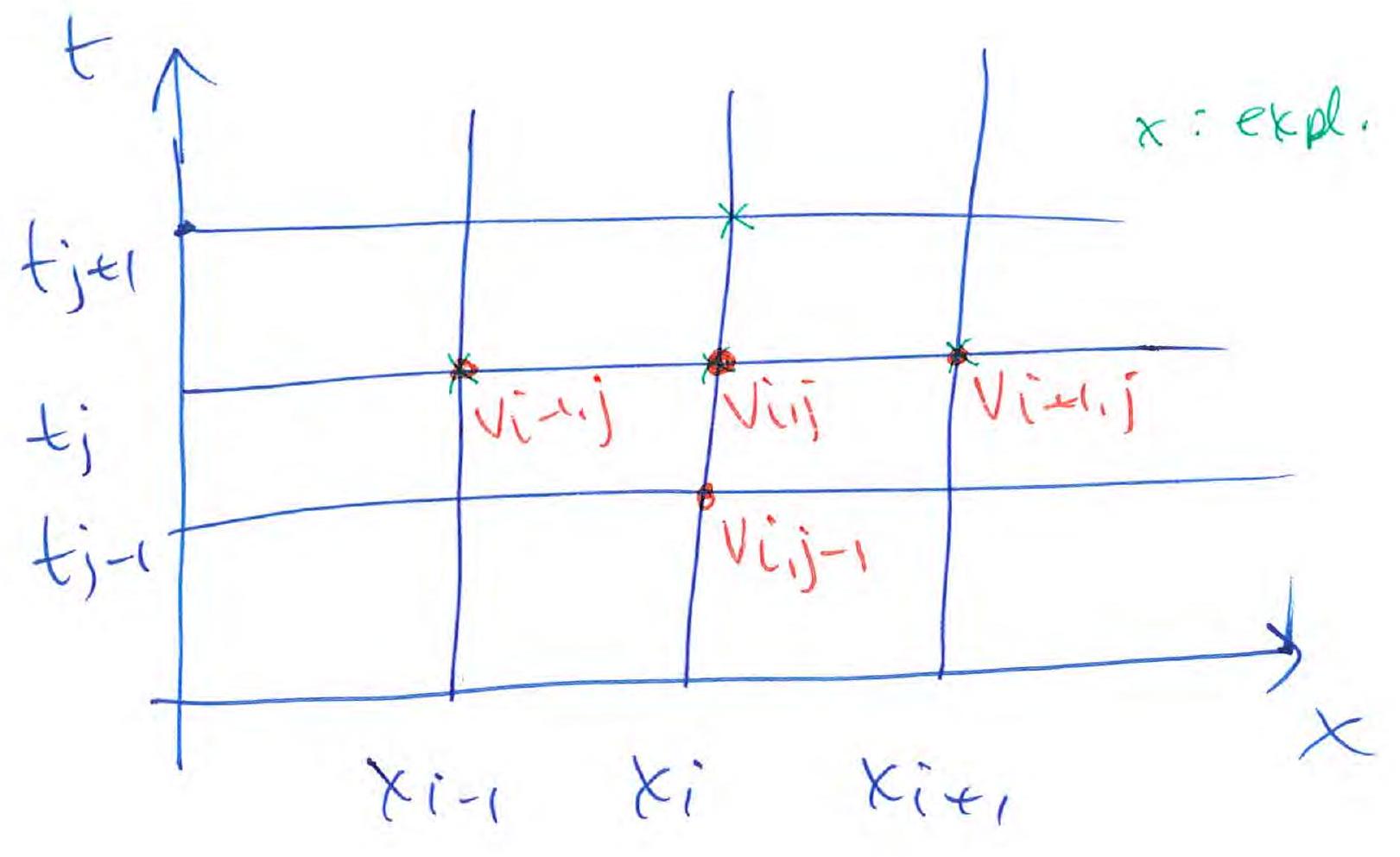
Finite difference method for diffusion PDE: explicit scheme

Equations: $\left(\alpha =\Delta t/\Delta x^2\right)$

$$\begin{array}{c}{v}_{1,j+1}=\alpha v_{0,j}+(1-2\alpha )v_{1,j}+\alpha v_{2,j}\\ ⋮\\ v_{i,j+1}=\alpha v_{i-1,j}+(1-2\alpha )v_{i,j}+\alpha v_{i+1,j}\\ ⋮\\ v_{n,j+1}=\alpha v_{n-1,j}+(1-2\alpha )v_{n,j}+\alpha v_{n+1,j}\end{array}$$

Solution at time step $t_{j+1}$ is explicitly expressed in terms of solution at time step $t_j$. That is, the explicit scheme is

$$\begin{array}{rl}{\mathbf{v}}_{j+1}& =\hat{A}{\mathbf{v}}_j\\ \Rightarrow {\mathbf{v}}_j& ={\hat{A}}^j{\mathbf{v}}_0\end{array}$$

where

$$\hat{A}=I-\alpha \hat{B},\hat{B}=\left[\begin{array}{cccc}2& -1& 0& 0\\ -1& 2& \ddots & 0\\ 0& \ddots & \ddots & -1\\ 0& 0& -1& 2\end{array}\right],{\mathbf{v}}_j=\left[\begin{array}{c}{v}_{1,j}\\ v_{2,j}\\ ⋮\\ v_{n,j}\end{array}\right]$$

Stability of the explicit scheme

The solution of $u_t=k{u}_{xx}$ goes to 0 when $t\to \infty$. Therefore, we should have

$$\begin{array}{rl}& \Vert {\vec{V}}_j\Vert =\Vert {\hat{A}}^j{\vec{V}}_0\Vert \underset{j\to \infty }{\to }0\\ & \iff \Vert {\hat{A}}^j\Vert \underset{j\to \infty }{\to }0\\ & \hat{A}=I-\alpha \hat{B}\\ & \hat{B}=\left[\begin{array}{ccc}2& -1& 0\\ -1& \ddots & -1\\ 0& -1& 2\end{array}\right]\end{array}$$

A result from linear algebra

A matrix $C$ is diagonalizable if we can write

$$\begin{array}{rl}C=R& D{R}^{-1}\end{array}$$

where $D$ is a diagonal matrix with the eigenvalues of $C$ on the diagonal.

Then,

$$c^n=\underset{n\text{ times }}{\underbrace{c\cdot c\cdots \cdots \cdot c}}$$ $$\begin{array}{rl}& =\underset{n\text{ times }}{\underbrace{\left(RD{R}^{-1}\right)\left(RD{R}^{-1}\right)\cdots \left(RD{R}^{-1}\right)}}\\ & =R\underset{=I}{D{R}^{-1}RD\underset{=I}{\underbrace{R^{-1}R}}RD\cdots \underset{=I}{\underbrace{R^{-1}RD{R}^{-1}}}}\\ & =R\underset{n\text{ times }}{\underbrace{D\cdot D\cdots D{R}^{-1}=R{D}^n{R}^{-1}}}\\ & =R\left[\begin{array}{ccc}{\lambda }_1^n& & \\ {\lambda }_2^n& O& \\ O& & {\lambda }_k^n\end{array}\right]R^{-1}\end{array}$$

It all $\lambda$ have $|\lambda |<1$, then $\Vert C^n\Vert \underset{n\to \infty }{\to }0$.

What are the eigenvalues of $\hat{A}=I-\alpha \hat{B}$? ($A\vec{v}=\lambda \vec{v}$: $\lambda$ is an eigenvalue.)

$$\hat{A}=I-\alpha \left[\begin{array}{ccc}2& -1& \\ -1& \ddots & -1\\ & -1& 2\end{array}\right]$$

We know that the eigenvalues of $\hat{B}$ are

$$\begin{array}{rl}& {\mu }_j=2-2\cos (j\theta ),\\ & \theta =\frac{\pi }{n+1},j=1,2,\dots ,n.\end{array}$$

Note that

$$0<{\mu }_j<4$$

Since the eigenvalues of $\hat{B}$ are $\mu$, the eigenvalues of $\hat{A}$ are $1-\alpha \mu$:

$$\begin{array}{rl}\hat{A}\vec{w}& =(I-\alpha \hat{B})\vec{w}\\ & =I\vec{w}-\alpha \hat{B}\vec{w}\\ & =1\cdot \vec{w}-\alpha \mu \vec{w}\\ & =\underset{\text{Eigenvalues of }\hat{A}}{\underbrace{(1-\alpha \mu )}}\vec{w}\end{array}$$

For stability we need $|\lambda |=\left|1-\alpha \mu \right|<1$:

$$\begin{array}{rl}& -1<1-{\alpha }_{\mu }<1\\ & 1-{\alpha }_{\mu }<1\\ & \iff -1<1-{\alpha }_{\mu }\\ & \Rightarrow \alpha \mu -1<1\\ & \alpha \mu <2\\ & \alpha <\frac{2}{\mu }\end{array}\text{\hspace{1em}(C)}$$

Specifically,

$$\begin{array}{rl}& \alpha <\min \left(\frac{2}{\mu }\right)\\ & =\frac{2}{\max \mu }=\frac{2}{4}\\ & \alpha <\frac{1}{2}\end{array}$$

Stability requirement for the explicit scheme.

$$\begin{array}{rl}& \frac{\Delta t}{\Delta x^2}<\frac{1}{2}\\ & \Delta t=\frac{1}{2}\Delta x^2\end{array}$$

Implicit scheme for the heat/diffusion PDE

PDE: $u_t=u_{xx}$ $u_{xx}\approx \frac{v_{i+1,j}-2v_{i,j}+v_{i-1,j}}{\Delta x^2}$ (same as in explicit scheme) $u_t\approx \underset{\text{Uses the solution at }{t}_j\text{ and }{t}_{j-1}}{\underbrace{\frac{v_{i,j}-v_{i,j-1}}{\Delta t}}}$

Discretized PDE:

$$\frac{V_{i,j}-V_{i,j-1}}{\Delta t}=\frac{V_{i+1,j}-2V_{i,j}+V_{i-1,j}}{\Delta x^2}$$

“Calculation molecule”: the scheme couples $v_{i,j-1}$ and $v_{i-1,j},v_{i,j},v_{i+1,j}$.

This gives us the scheme

$$\begin{array}{rl}{\vec{V}}_{j-1}& =\tilde{A}{\vec{V}}_j\\ \tilde{A}& =I+\alpha \hat{B}\\ & =\left[\begin{array}{cccc}1+2\alpha & -\alpha & & \\ -\alpha & 1+2\alpha & 0& \\ 0& & \ddots & -\alpha \\ & & -\alpha & 1+2\alpha \end{array}\right]\\ \Rightarrow {\tilde{A}}^{-1}{\vec{V}}_{j-1}& ={\tilde{A}}^{-1}\tilde{A}{\vec{V}}_j\\ \Rightarrow {\vec{V}}_j& ={\tilde{A}}^{-1}{\vec{V}}_{j-1}\text{(implicit)}\end{array}$$ $$\begin{array}{rl}{\vec{V}}_j& ={\tilde{A}}^{-1}{\vec{V}}_{j-1}\\ \Rightarrow {\vec{V}}_j& ={\left({\tilde{A}}^{-1}\right)}^j{\vec{V}}_0\end{array}$$

Numerical solution of implicit scheme Is this scheme stable? $\tilde{A}=I+\alpha \hat{B}$ has eigenvalues $1+\alpha \mu$, where $0<\mu <4$.

All eigenvalues of $\tilde{A}$ are > 1.

Reminder:

$$\begin{array}{rl}& M\vec{w}=\lambda \vec{w}:\lambda \text{ are eigenvalues of }M\\ & \Rightarrow \underset{I}{\underbrace{M^{-1}M}}\vec{w}=M^{-1}\lambda \vec{w}\\ & \Rightarrow \lambda \cdot M^{-1}\vec{w}=\vec{w}\\ & M^{-1}\vec{w}=\frac{1}{\lambda }\vec{w}\end{array}$$

Eigenvalues of $M^{-1}$ are $\frac{1}{\lambda }$.

Thus, ${\tilde{A}}^{-1}$ has the eigenvalues $\frac{1}{1+\alpha \mu }<1$ such that all eigenvalues of ${\tilde{A}}^{-1}$ satisfy

$$|\lambda |<1.$$

The implicit scheme is stable, regardless of the value of $\alpha$.

Crank-Nicolson scheme

Approximations: $u_t\left(x_i,t_j\right)\approx \frac{v_{i,j}-v_{i,j-1}}{\Delta t}$ (same as in the implicit scheme) $u_{xx}\left(x_i,t_j\right)$ $\approx \theta \frac{v_{i-1,j}-2v_{i,j}+v_{i+1,j}}{\Delta x^2}$ (at $t=t_j$) $+(1-\theta )\frac{V_{i-1,j-1}-2V_{i,j-1}+V_{i+1,j-1}}{\Delta x^2}$

Weighted average of the approximations to $u_{xx}$ at $t=t_j$ and $t=t_{j-1}$.

Taylor-expanding these expressions at $\left(x_i,t_j-\Delta t/2\right)$, we get $\frac{V_{i,j}-V_{i,j-1}}{\Delta t}=u_t\left(x_i,t_j-\frac{\Delta t}{2}\right)+\underset{\text{error term}}{\underbrace{C\Delta t^2}}$ Similarly, if $\theta =\frac{1}{2}$: $\frac{1}{2}\frac{v_{i-1,j}-2v_{i,j}+v_{i+1,j}}{\Delta x^2}$ $+\frac{1}{2}\frac{v_{i-1,j-1}-2v_{i,j-1}+v_{i+1,j-1}}{\Delta x^2}$ $=\dots =u_{xx}\left(x_i,t_j-\frac{\Delta t}{2}\right)+\underset{\text{error term }}{\underbrace{C\Delta x^2}}$

The C–N scheme with $\theta =\frac{1}{2}$ gives a second order error in both $\Delta t$ and $\Delta x$ at $t=t_j-\frac{\Delta t}{2}$. C–N scheme for $\theta =\frac{1}{2}$:

$$\begin{array}{rl}& (2I+\alpha \hat{B}){\vec{V}}_j=(2I-\alpha \hat{B}){\vec{V}}_{j-1}\\ \iff & \underset{\text{C–N scheme}}{\underbrace{{\vec{V}}_j=(2I+\alpha \hat{B}{)}^{-1}(2I-\alpha \hat{B}){\vec{V}}_{j-1}}}\\ \Rightarrow & {\vec{V}}_j={\left[(2I+\alpha \hat{B}{)}^{-1}(2I-\alpha \hat{B})\right]}^j{\vec{V}}_0\end{array}$$

Is this scheme stable? Eigenvalues of $(2I+\alpha \hat{B}{)}^{-1}(2I-\alpha \hat{B})$:

$$\begin{array}{rl}& (2I\pm \alpha \hat{B})\vec{w}=2\vec{w}\pm \alpha \hat{B}\vec{w}\\ & =2\vec{w}\pm \alpha \mu \vec{w}\\ & =\underset{\text{Eigenvalues of }2I\pm \alpha \hat{B}}{\underbrace{(2\pm \alpha \mu )\vec{w}}}\\ & (2I+\alpha \hat{B}{)}^{-1}(2I-\alpha \hat{B})\vec{w}\\ & =(2-\alpha \mu )(2I+\alpha \hat{B}{)}^{-1}\vec{w}\\ & =\frac{2-\alpha \mu }{2+\alpha \mu }\vec{w}\end{array}$$

So, eigenvalues of $(2I+\alpha \hat{B}{)}^{-1}(2I-\alpha \hat{B})$ are

$$\lambda =\frac{2-\alpha \mu }{2+\alpha \mu }$$

We have

$$\begin{array}{rl}\lambda & =\frac{2+\alpha \mu -2\alpha \mu }{2+\alpha \mu }\\ & =1-2\frac{\alpha \mu }{2+\alpha \mu }\text{(between −1 and 1)}\end{array}$$

This is $<1$ and $>-1$ :

$$|\lambda |<1$$

Scheme is stable for all $\alpha$.

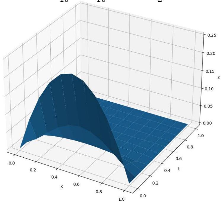
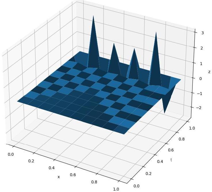
Numerical solution obtained using the explicit scheme

$$\Delta t=\frac{1}{10},\Delta x=\frac{1}{10}\Rightarrow \alpha =10>\frac{1}{2}$$

$$\Delta t=\frac{1}{400},\Delta x=\frac{1}{10}\Rightarrow \alpha =\frac{1}{4}<\frac{1}{2}$$

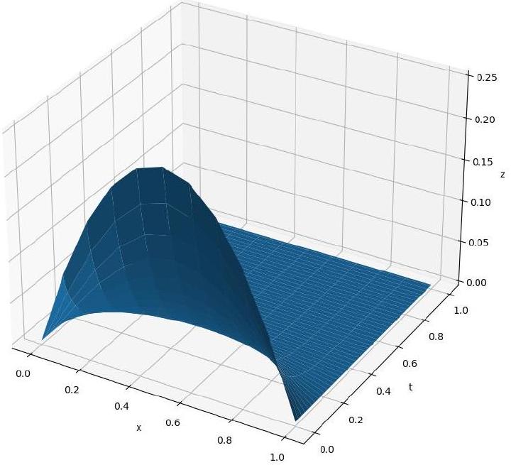
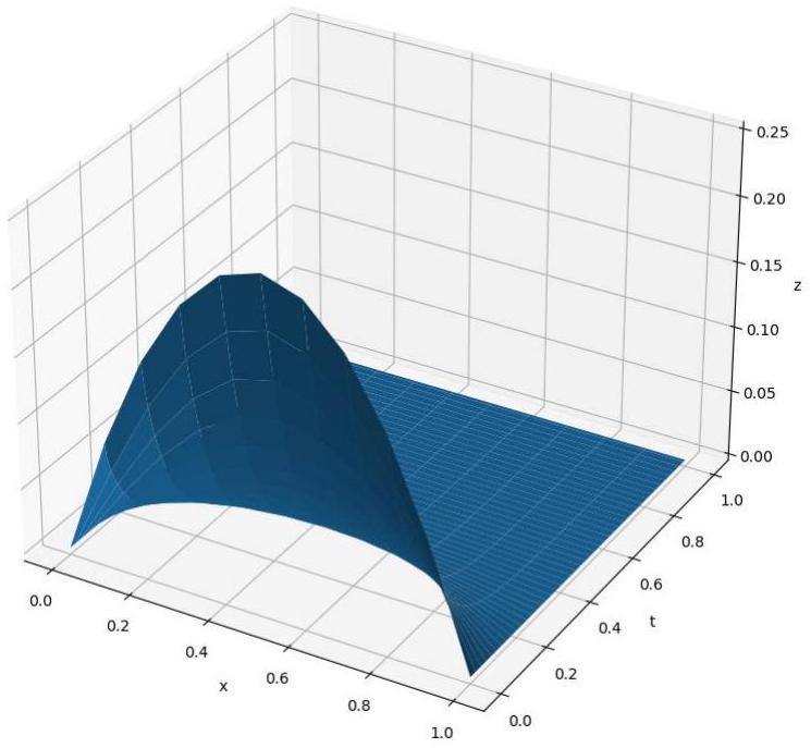
Numerical solution obtained using the implicit scheme

$$\Delta t=\frac{1}{10},\Delta x=\frac{1}{10}\Rightarrow \alpha =10>\frac{1}{2}$$

$$\Delta t=\frac{1}{400},\Delta x=\frac{1}{10}\Rightarrow \alpha =\frac{1}{4}<\frac{1}{2}$$

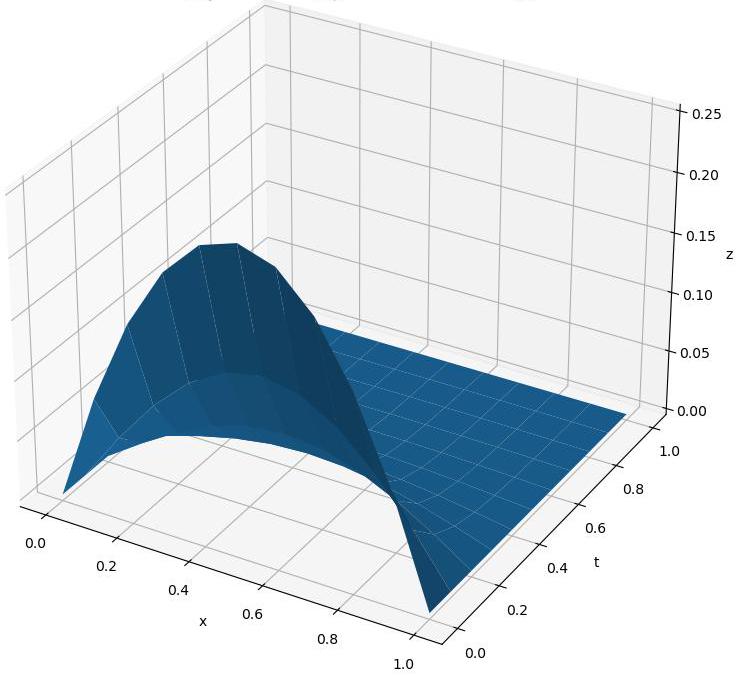
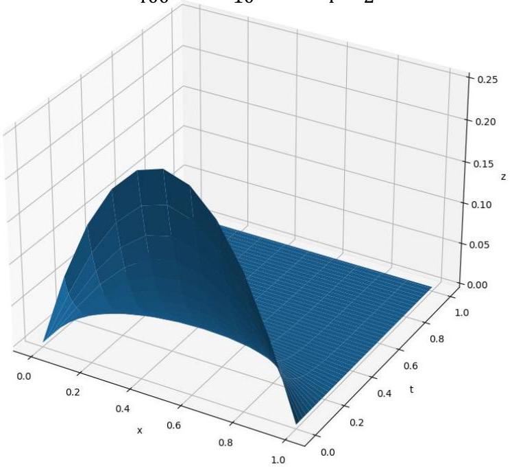
Numerical solution obtained using the C-N-scheme

$$\Delta t=\frac{1}{10},\Delta x=\frac{1}{10}\Rightarrow \alpha =10>\frac{1}{2}$$

$$\Delta t=\frac{1}{400},\Delta x=\frac{1}{10}\Rightarrow \alpha =\frac{1}{4}<\frac{1}{2}$$