PENG9570 — Lecture 3 (February 26th)
Phase line plots
Bifurcations
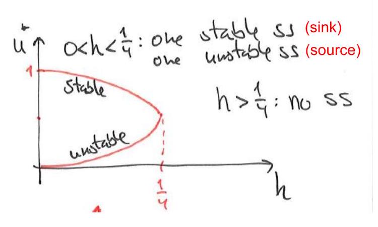
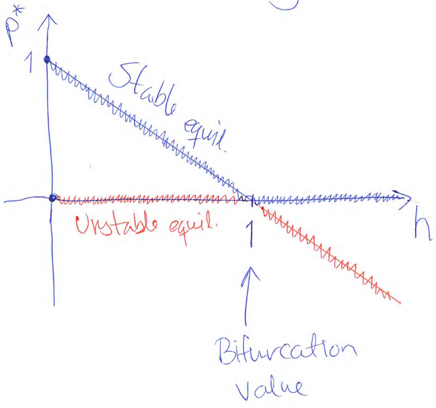
Bifurcation diagram:
Problem
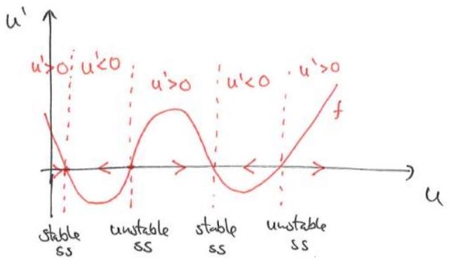
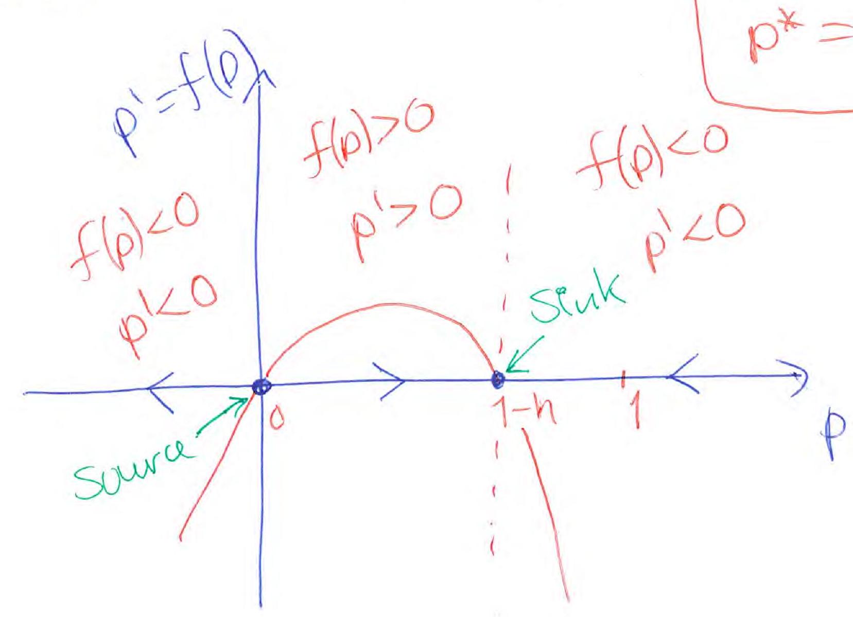
- Sketch the phase line plot of
for different values of the parameter .
- Identify stable and unstable equilibria (sinks and sources).
Example
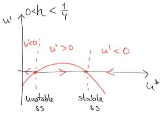
Phase line plot of
Equilibria (): and .
I. :
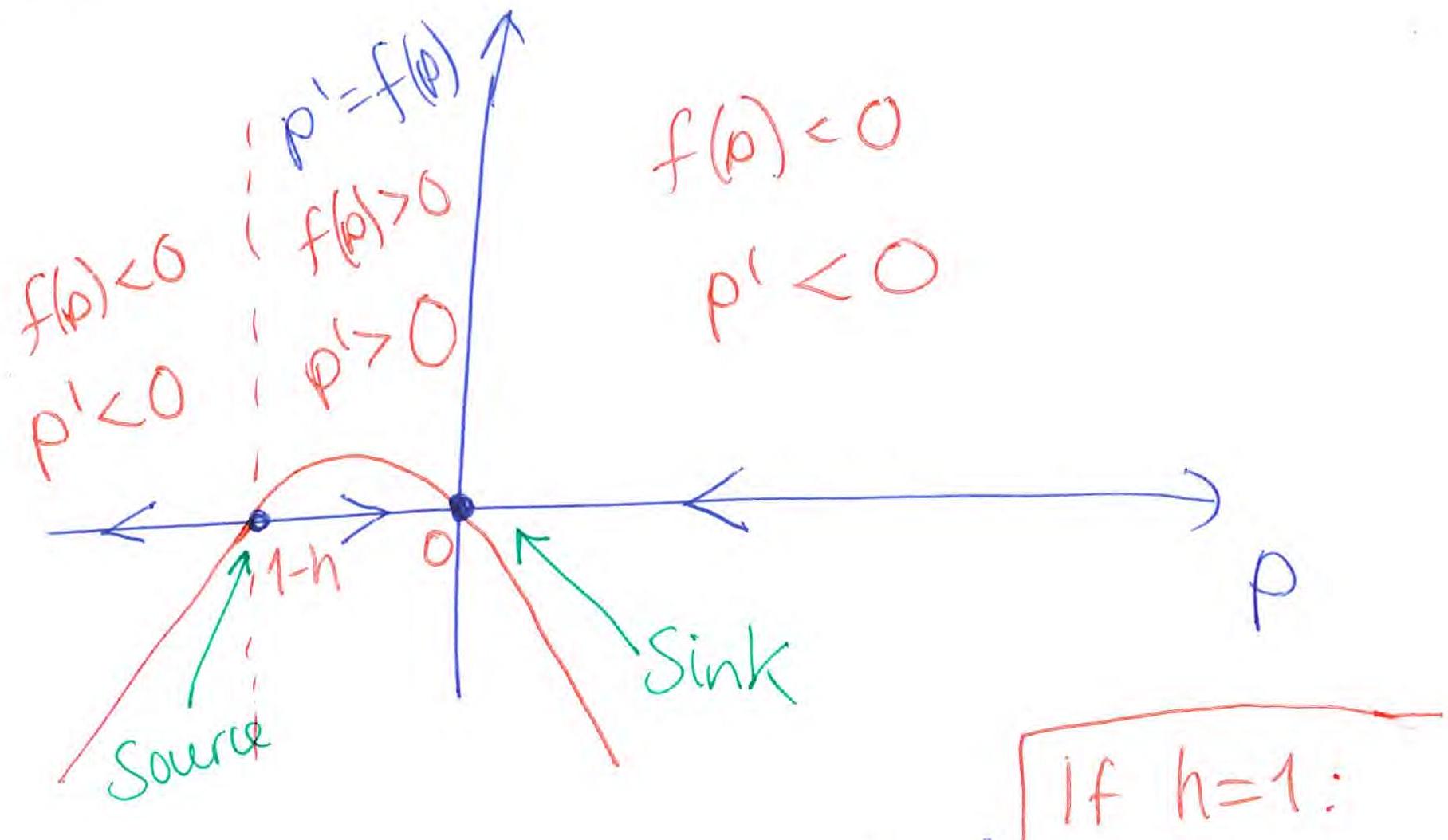
II. :
(If : , .)
Bifurcation diagram:
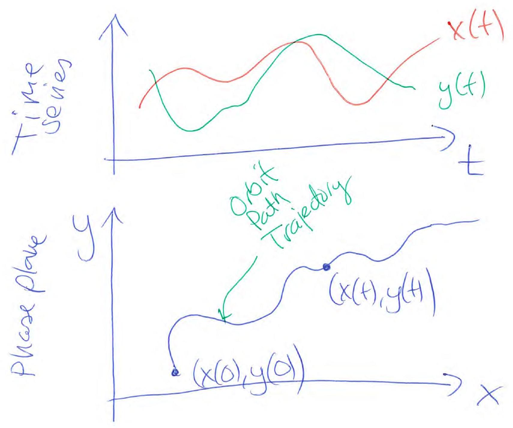
Two-variable ODE systems
Solution curves:
Example
Characteristic polynomial:
General solution
Alternatively: Introduce . Then
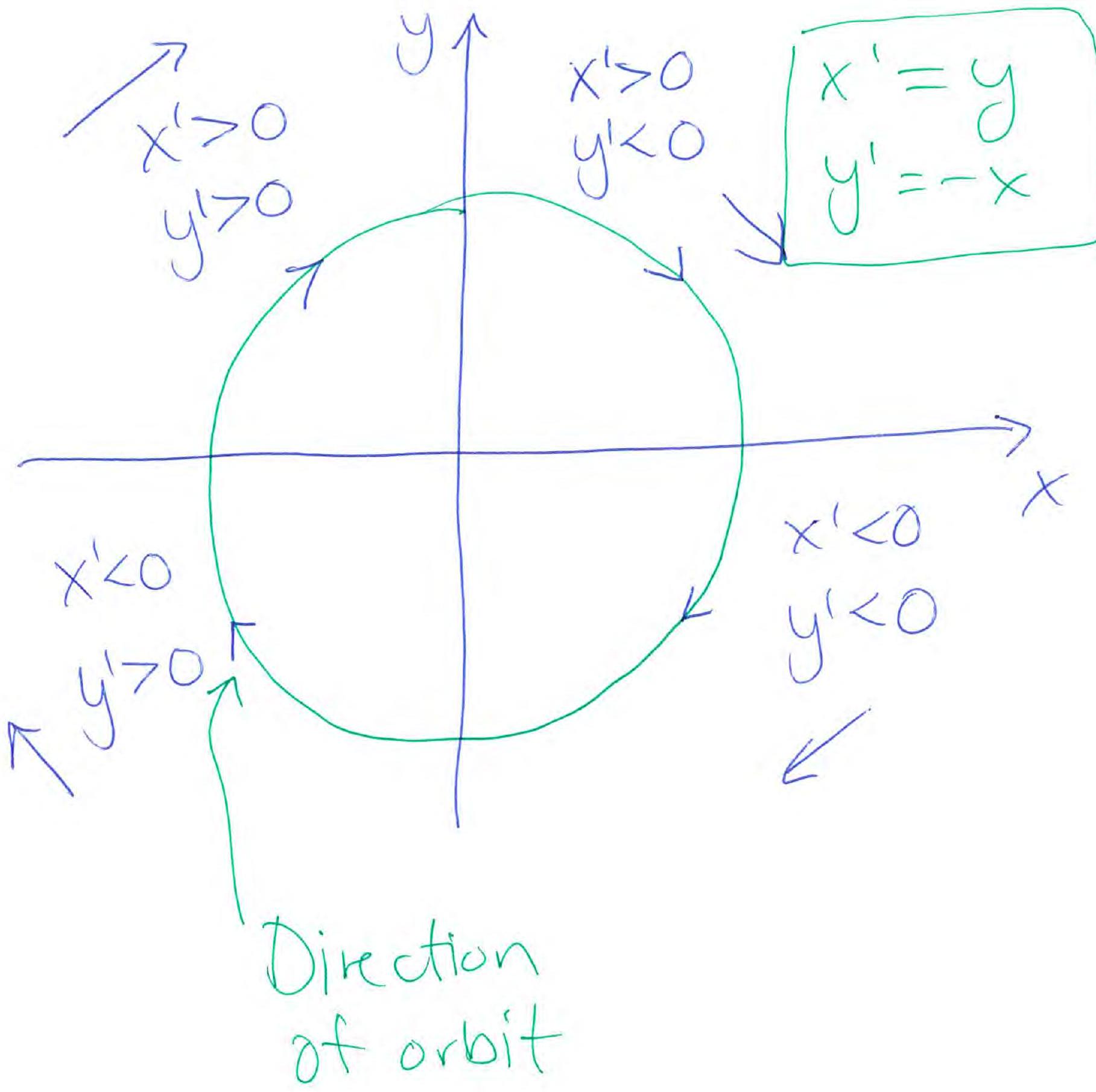
System of ODEs:
We know that
Then,
(Separable ODE)
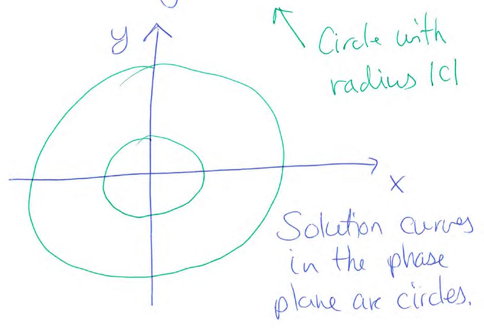
I.e. circles with radius . 3.
Derivative of is zero means
Solution curves are circles with radius .
Linear systems of ODEs
( are constants.) Coefficient matrix:
Assumption: is non-singular. System in matrix–vector form:
Solution
We look for solutions of the form
Inserting this into we get:
Here is an eigenvalue of and the corresponding eigenvector. Non-trivial solutions require
For :
Three different types of solution pairs:
I. Two real and unequal ‘s II. One real (skipped) III. Two complex conjugate ‘s:
Case I
are both real and . Assume and are the corresponding eigenvectors. Then,
Case III
, , with . The vectors and are the corresponding eigenvectors. Then, using Euler’s formula :
Types of equilibria
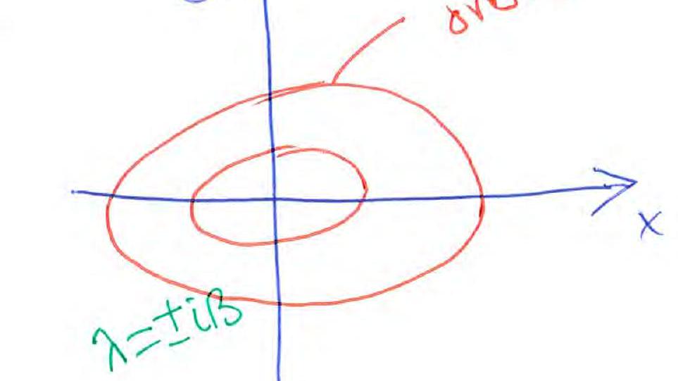
Center:

- Source: all orbits move away from .
- Sink: all orbits approach as (or as for a source).
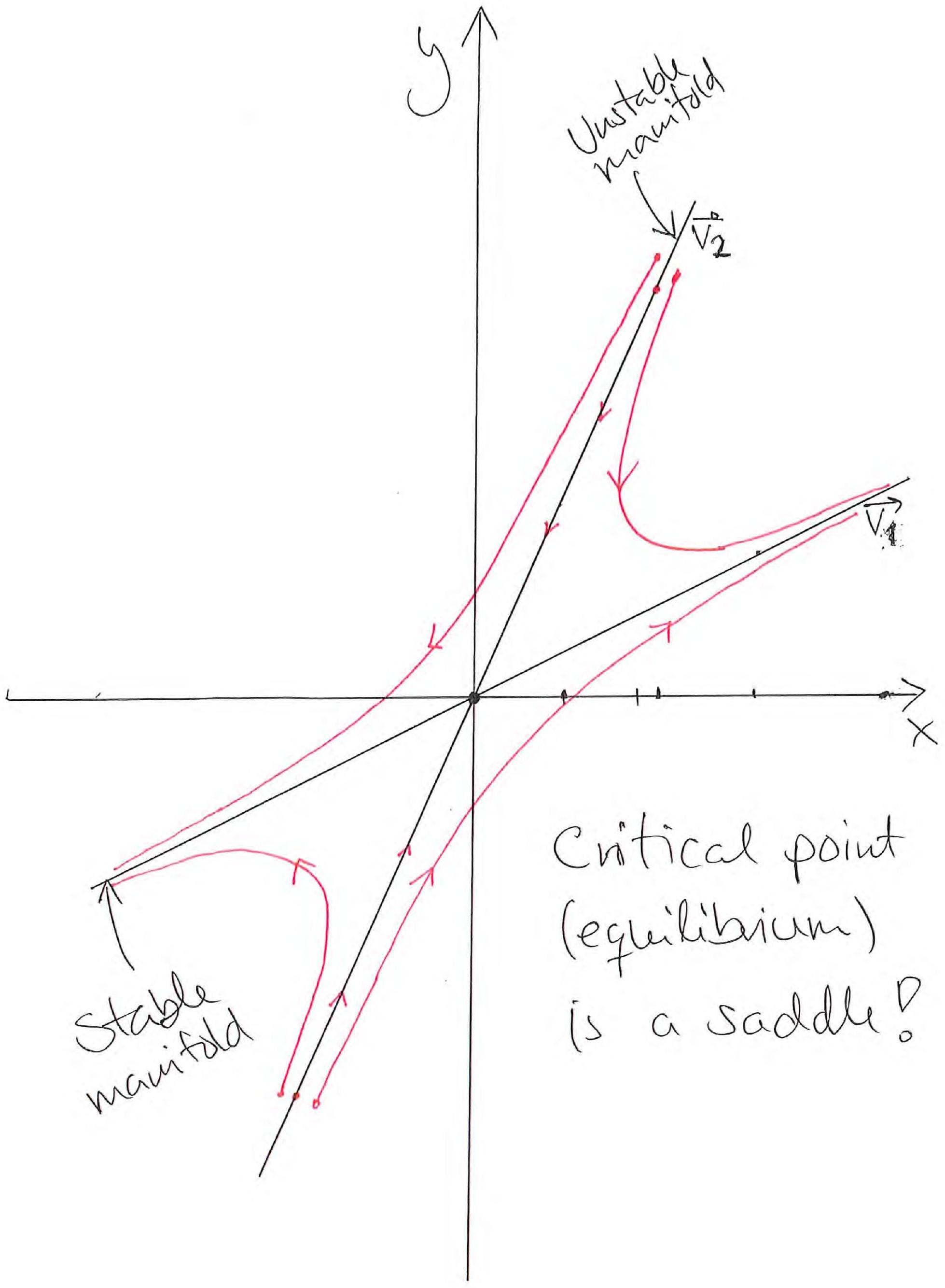
- Saddle (node): orbits approach except for orbits on the unstable manifold.
Example
Characteristic equation:
Real eigenvalues: one positive, one negative — a saddle equilibrium.
Eigenvector corresponding to :
We choose
Similarly we find
The general solution:
Nonlinear systems of ODEs
Assume that is an equilibrium: at , that is
Reminder: linearisation
The linearisation of a function at is
The linearisation of a function at is
This means that, near ,
To simplify we redefine variables:
Using these approximations we get the linearised system
where the Jacobian of the ODE system is
Does the linearised system behave in the same way as the nonlinear system near the equilibrium? Yes, but with one limitation. The Hartman–Grobman theorem states that if are not pure imaginary numbers, then the orbits of the original system near the equilibrium behave the same way as orbits of the linearised system near the equilibrium.
Example
Equilibrium: . Linearisation:
Jacobian:
Eigenvalues of :
Purely imaginary eigenvalues of the Jacobian, so the Hartman–Grobman theorem does not apply.
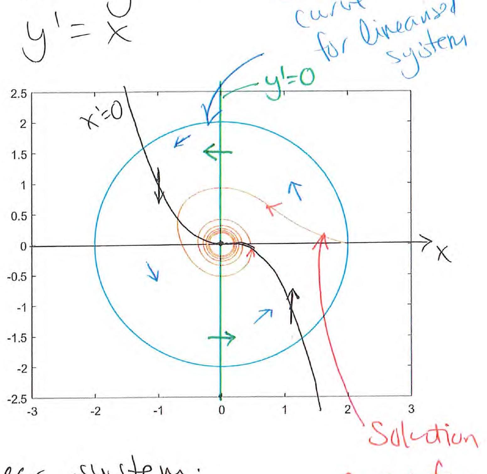
- Linear system: center at .
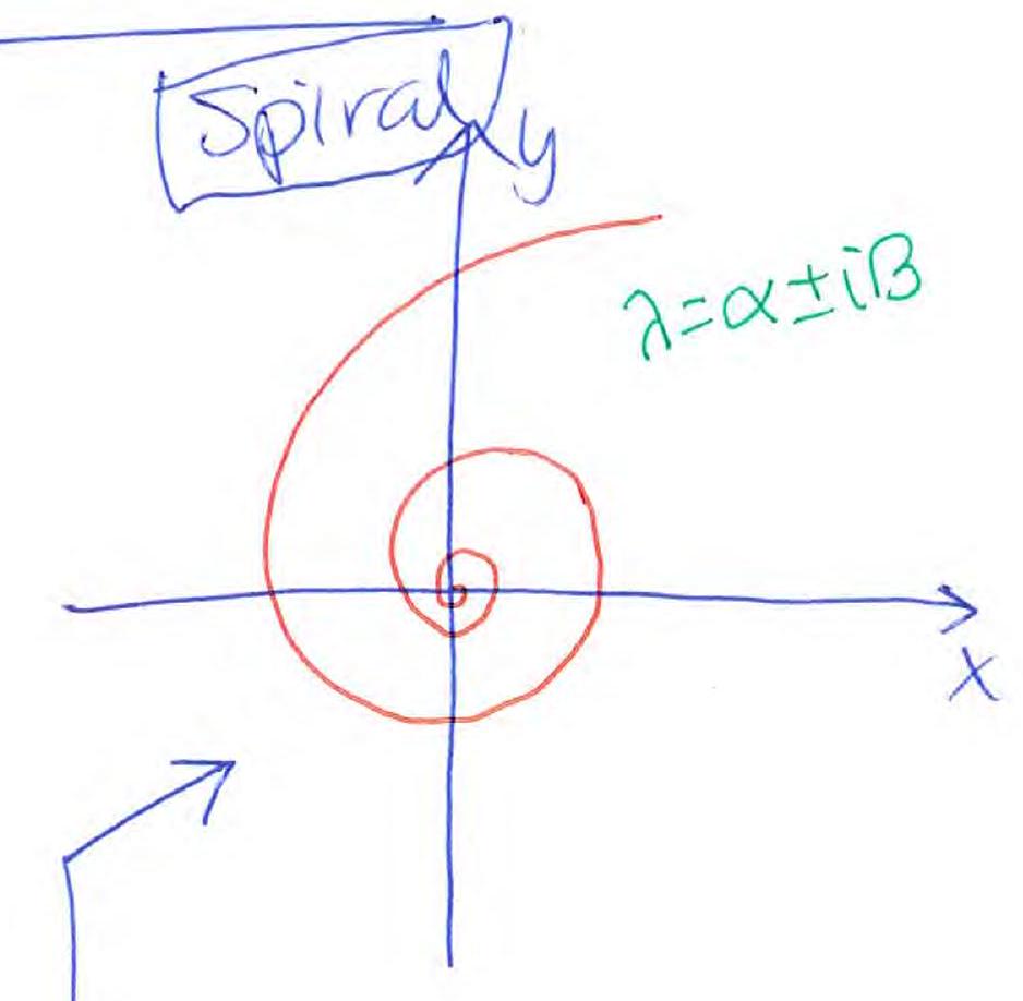
- Nonlinear system: stable spiral at .
Nullclines
The nullclines of a system of ODEs are the curves obtained when and are set equal to zero:
Example
Nullclines of
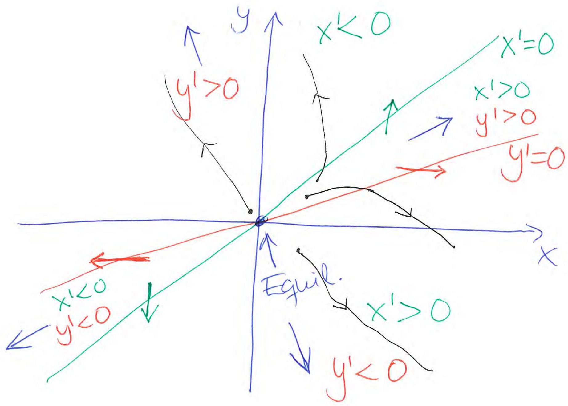
is an unstable equilibrium.