PENG9570 — Lecture 2 (February 25th)
Slope fields
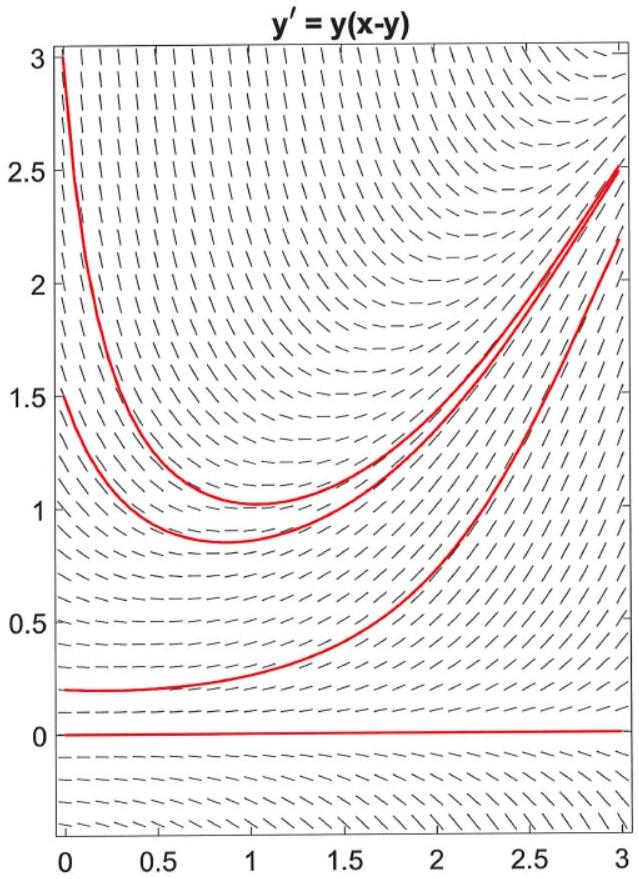
Slope field (direction field)
- Differential equation:
- The derivative is the slope of the tangent of the solution curve
- A slope field is defined by the magnitude of the derivatives, indicated by short straight lines
- An ODE has (most often) infinitely many solutions
The initial value problem
Normally one solution per initial value!
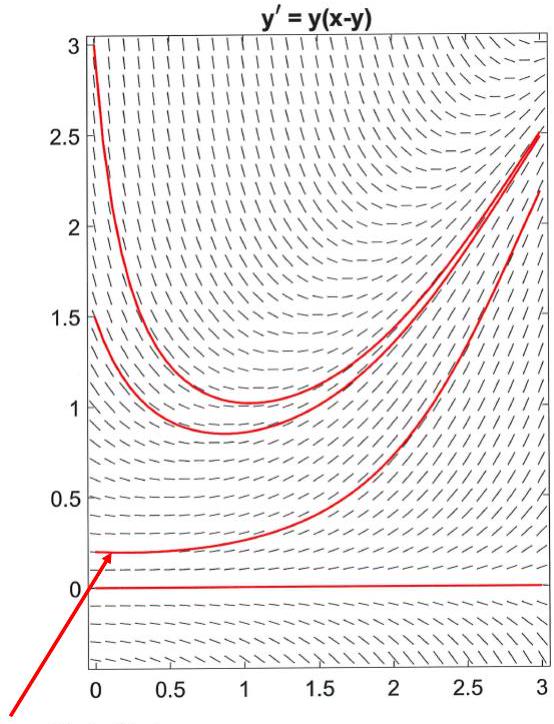
Solution with initial condition .
Slope fields, problem
Which of the following ODEs would produce the slope field shown below?
- A.
- B.
- C.
- D.
- E.
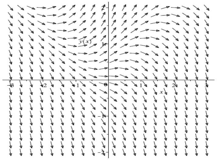
(On the slide, options A, B, D and E are crossed out; the answer is C.)
ODEs: stability and bifurcations
First-order, autonomous, one-variable ODE.
Equilibria are points where
(aka steady states, critical points, stationary points). Equilibria are calculated using this equation.
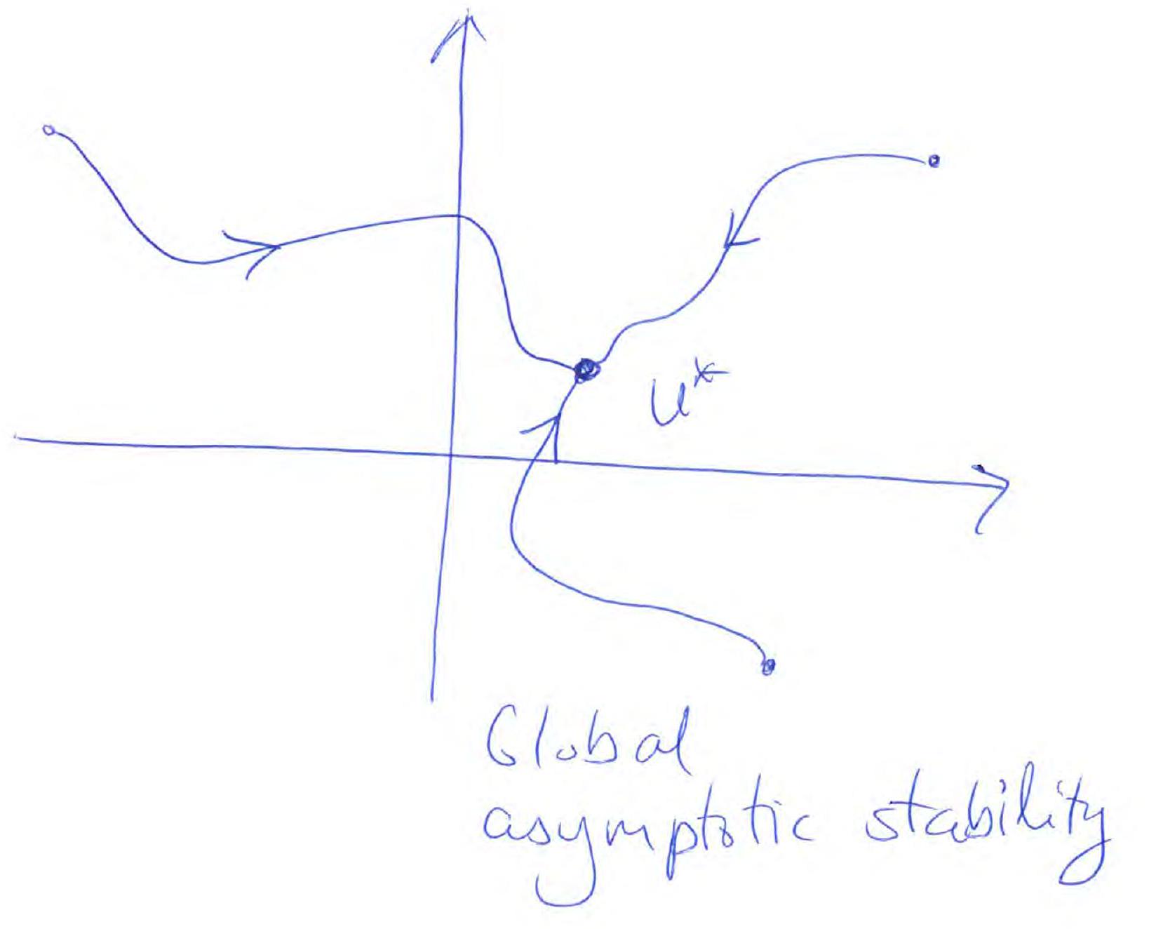
Equilibria: sinks and sources
Three types:
- Sinks (a.k.a. attractors or asymptotically stable equilibria)
- Sources (a.k.a. repellors or unstable equilibria)
- Nodes (semistable equilibria)
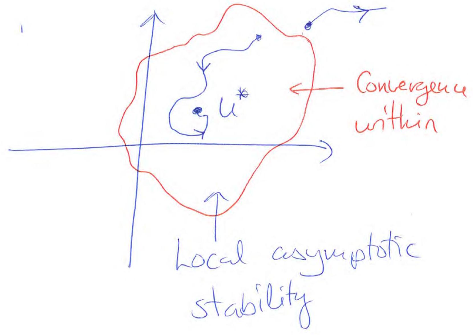
Definition
If is initially “close enough” to the sink and if , then is a locally asymptotically stable equilibrium (i.e. a sink).
Slope field of :
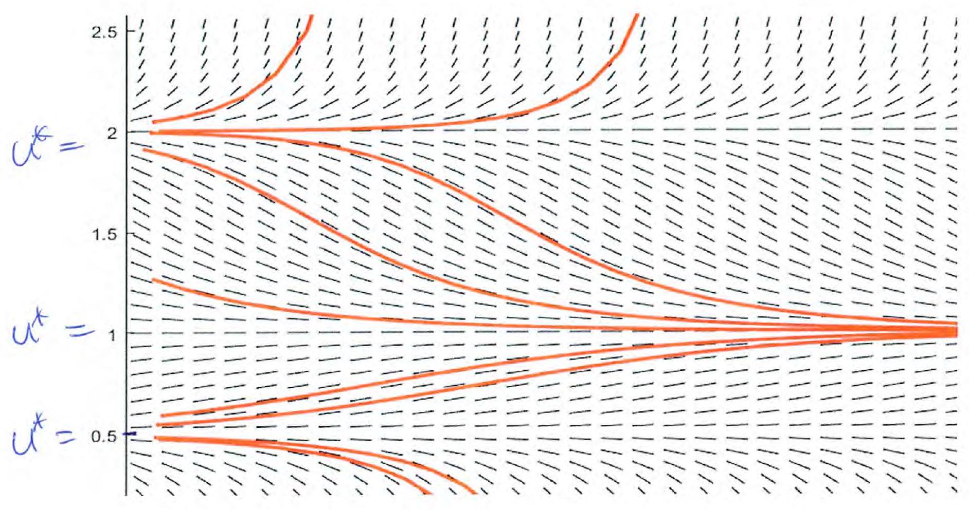
- : unstable equilibrium (source)
- : locally asymptotically stable equilibrium (sink)
- : unstable equilibrium (source)
Criterion for asymptotic stability
We introduce by
(Note that .) Then, by linearisation:
For to converge to , we need as . This requires as .
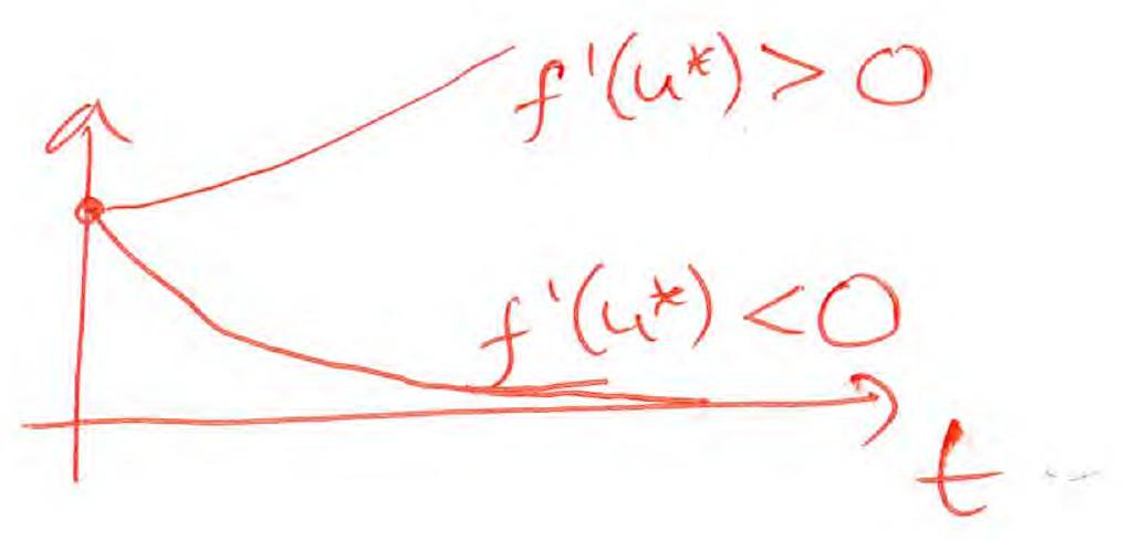
as when .
Asymptotic stability when .
An equilibrium from which escapes as is unstable and is called a source (or a repellor). A node is a sink or a source depending on circumstances; it is sometimes called a semistable equilibrium.
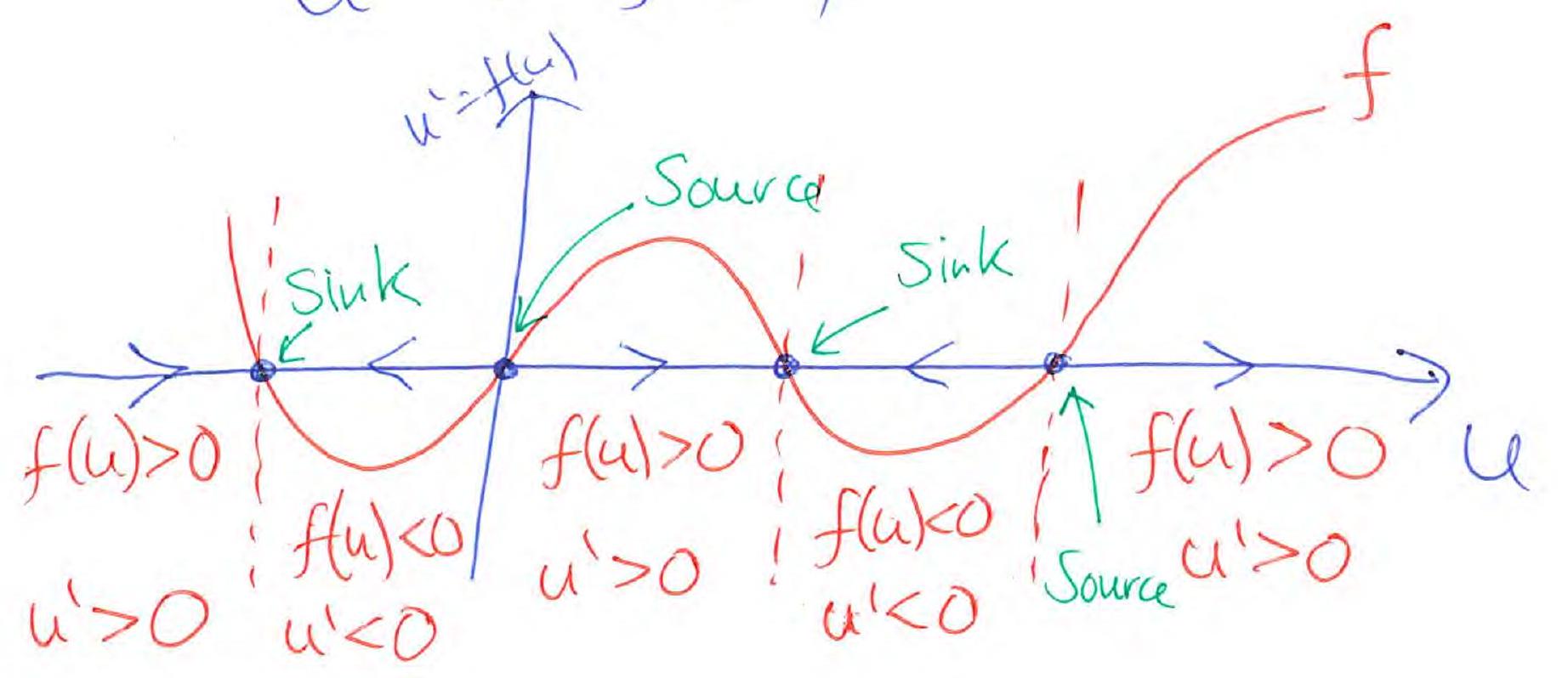
Phase line plots
Phase line plots show the graph of (where ) together with arrows that point in the direction in which the solution grows.
Example:
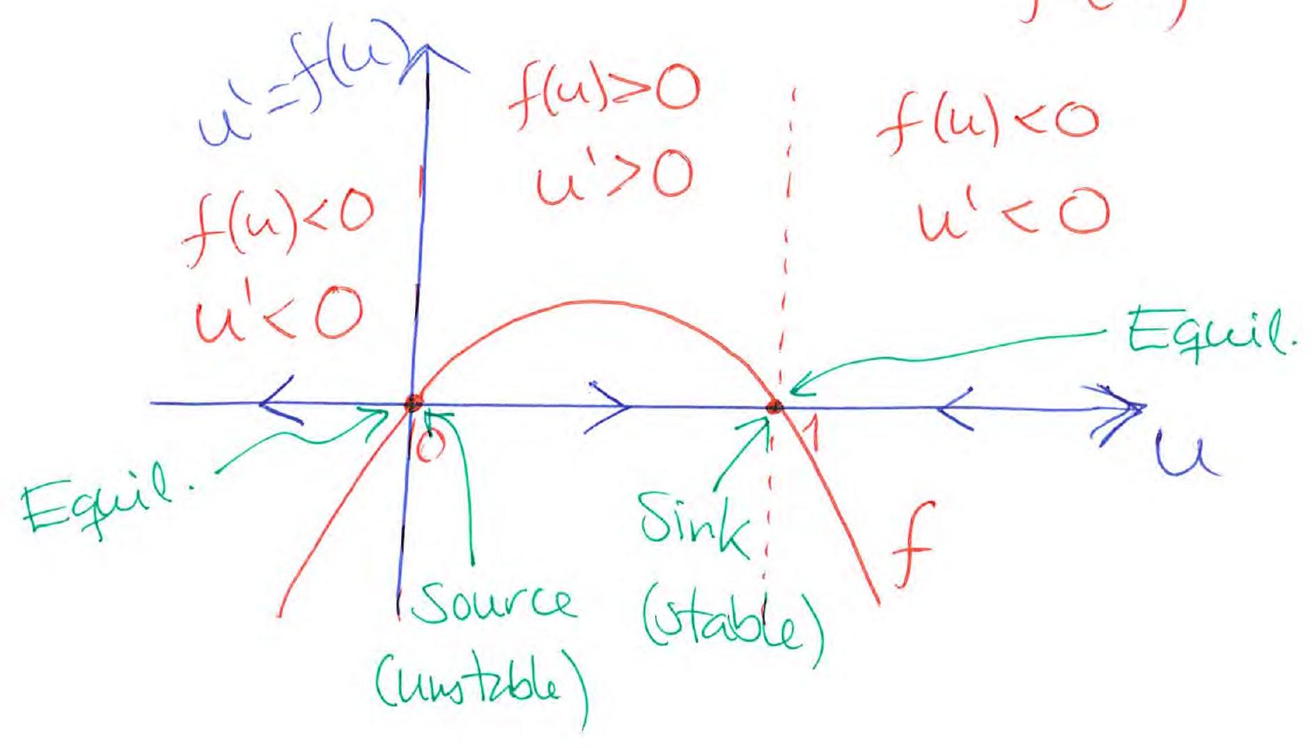
Generic phase line plot:
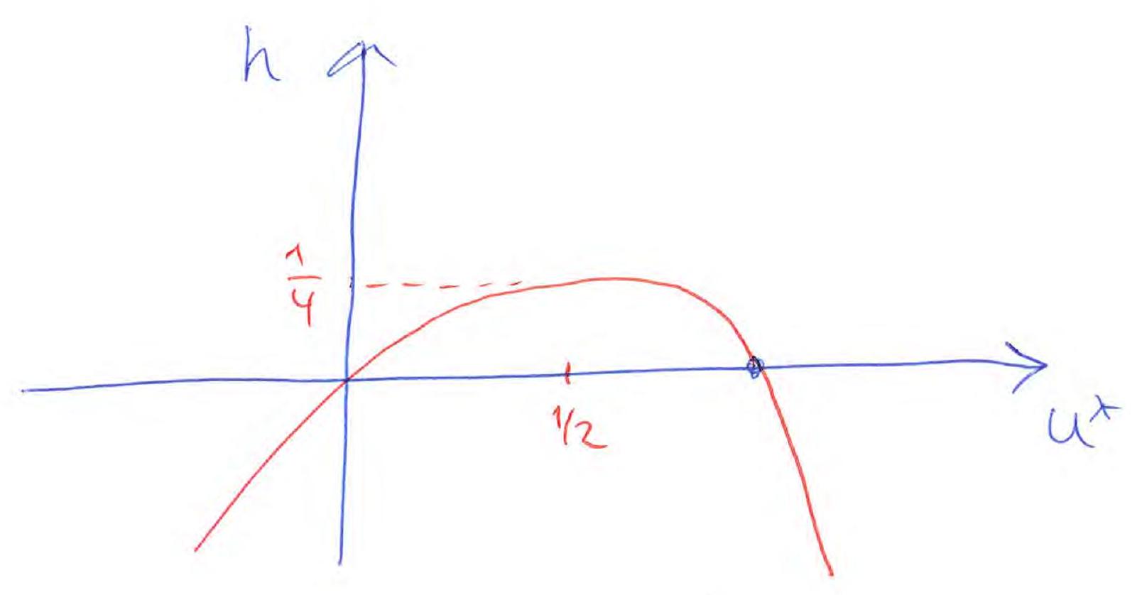
Example: logistic growth with harvesting
Scaling (dimensionless):
Scaled ODE:
Equilibria ():
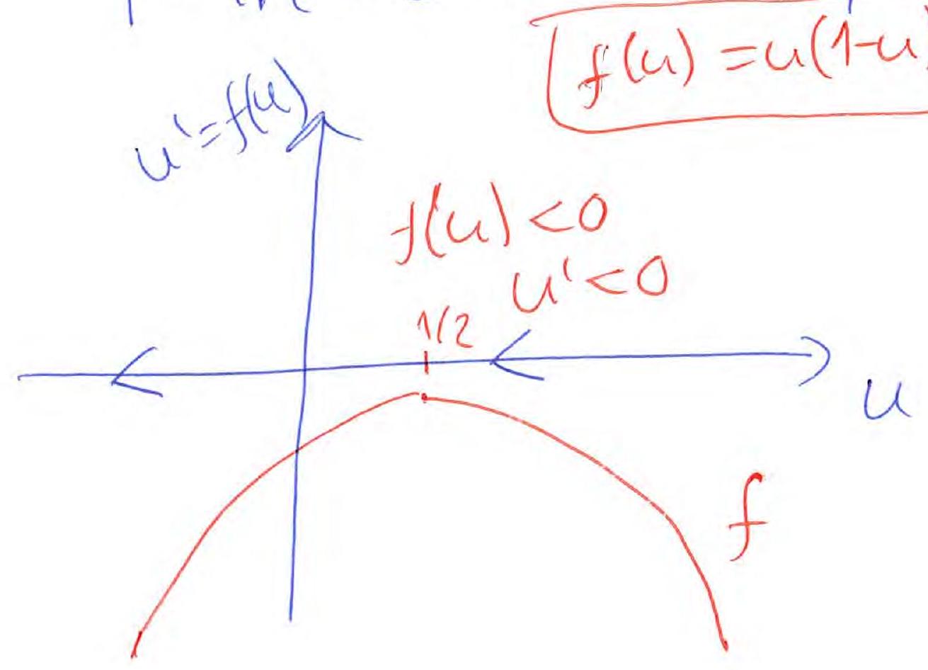
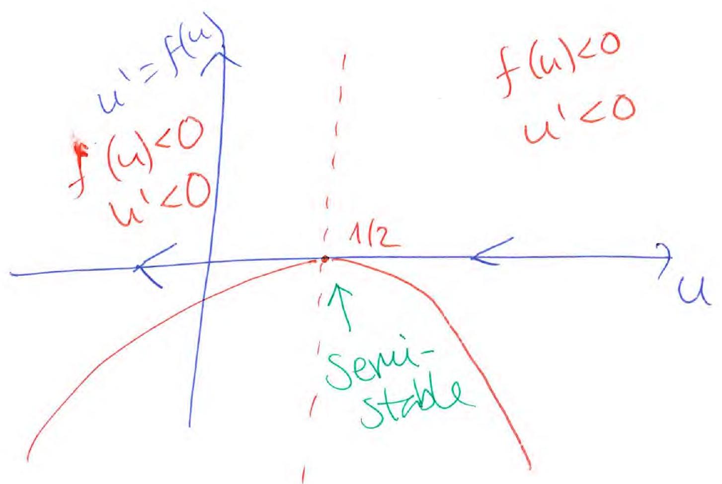
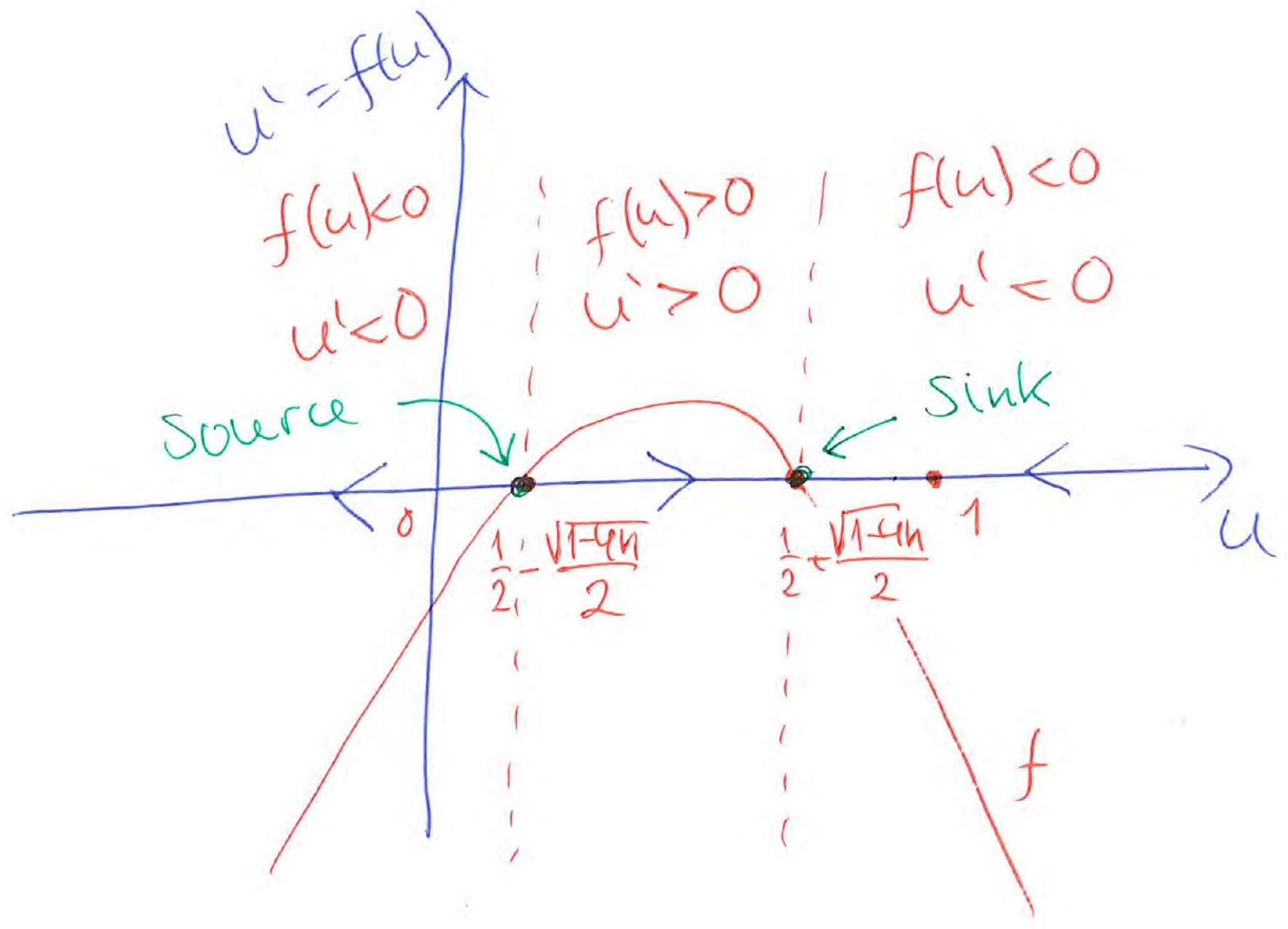
Three cases:
I. : no equilibrium II. : one equilibrium III. : two equilibria
Phase line plots:
I.
II.
III.
Visualising the dependence on the parameter — the bifurcation diagram
Equilibria and are related by
Change axes:
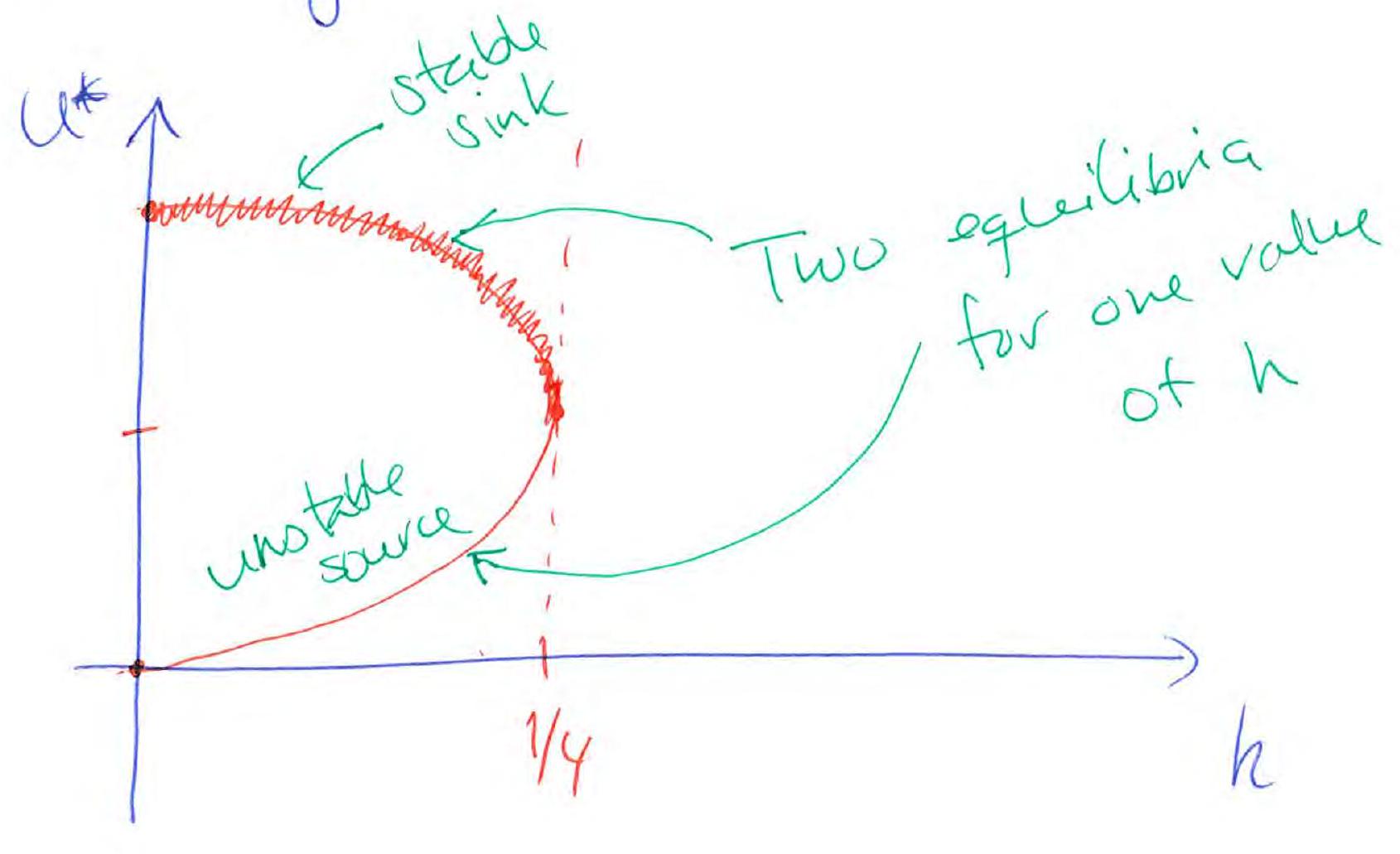
Bifurcation diagram for the logistic model with harvesting.