PENG9570 Lecture 1

Welcome to PENG9570

Applied Mathematical Modelling and Analysis Leiv Øyehaug — OsloMet (Oslo Metropolitan University)

Practical information

• Lecturers: Leiv Øyehaug (course responsible) and Sølve Selstø
• Course plan: https://student.oslomet.no/studier/studieinfo/emne/PENG9570/2025/HØST

Teaching sessions

Uke 10, 2026:

Time	Mon 9/3	Tue 10/3	Wed 11/3	Thu 12/3	Fri 13/3
08:00–10:00		Practical information; project	Lecture 08:30–10:15, Rom P35 PI243 (L. Øyehaug)	Lecture 08:30–12:15, Rom P35 U1007 (L. Øyehaug)	Lecture 08:30–12:15, Rom P35 PI243 (L. Øyehaug)

Project and exam

• Project:
  • As much of the syllabus as possible should be applied in the project (e.g. modelling, analysis, numerical solution)
  • Deadline for project report submission: June 1st
  • Report has to be approved for the candidate to take the exam
• Oral exam:
  • Presentation of project, including questions
  • Questions from the syllabus
  • Pass / no pass (Pass $\ge$ B!)
  • June 15th

Canvas

• Canvas page for the course: https://oslomet.instructure.com/courses/33405
• All course material will be made available here

Literature

• HJ Ricardo [HJR]: A Modern Introduction to Differential Equations, 3rd ed. (chapters 1–3, 6, 7): https://www.sciencedirect.com/book/monograph/9780128234174/a-modern-introduction-to-differential-equations
• Compendiums (homemade, see Canvas)
• Morten Hjorth-Jensen: Computational Physics (with permission, link in Canvas)
• Lecture notes

About me

• Leiv Øyehaug
• Associate professor of applied mathematics, Department of Computer Science
• Background mainly in modelling biological systems
• E-mail: leiv.oyehaug@oslomet.no
• Office: P35-PS234

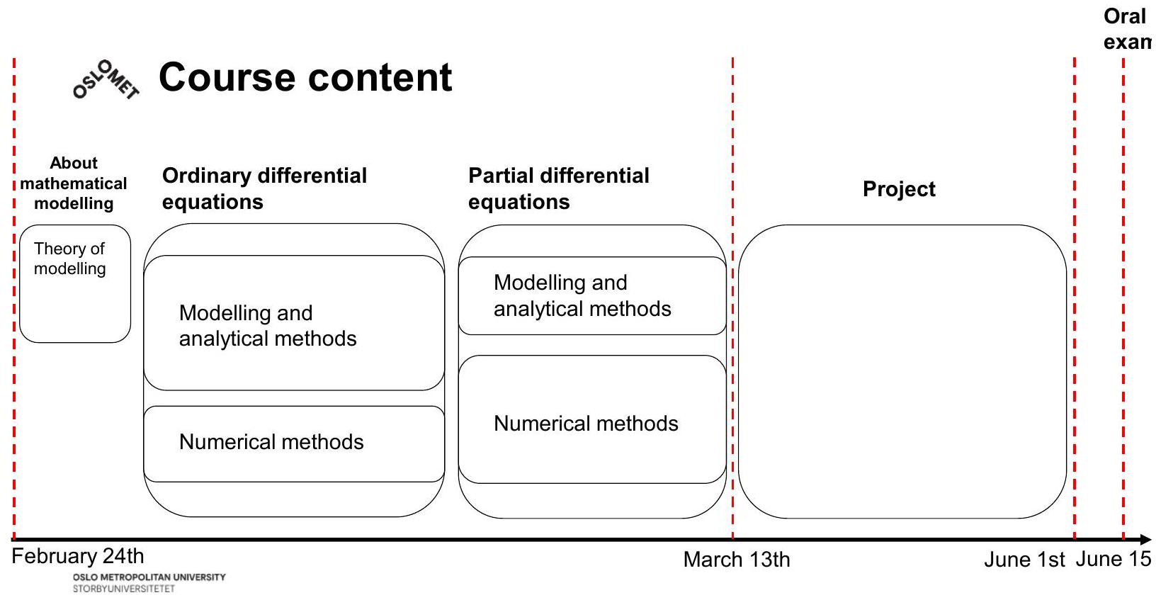
Main topics of the course

Analysis of ODEs — Lectures 1 & 2

Analysis of ODE systems — Lectures 2 & 3

Numerical methods for ODEs — Lectures 3 & 4

Introduction to PDEs — Lecture 4

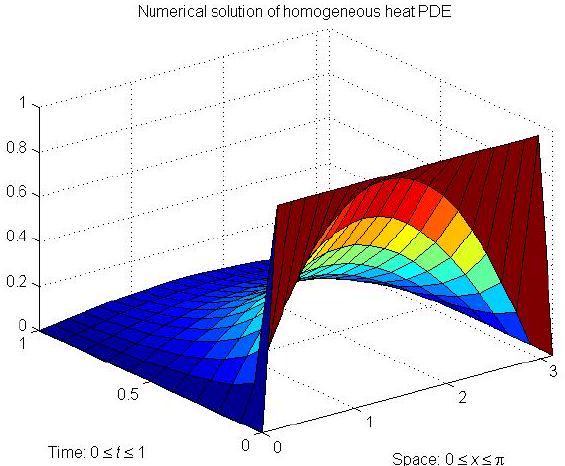
Numerical methods for PDEs — Lectures 5 & 6

Numerical methods for quantum physics — Lecture 7

$$i\hslash \frac{\partial }{\partial t}|\Psi ⟩=\hat{H}|\Psi ⟩$$

Summary

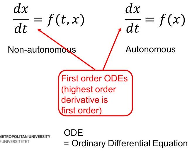
What is an ordinary differential equation (ODE) and what is an initial value problem?

An ordinary differential equation is an equation that relates a function $y$, its derivatives $y^{\prime },y^{\prime \prime },\dots$ and an independent variable (in this case $t$):

$$F\left(t,y,y^{\prime },\dots ,y^{(n)}\right)=0$$

An initial value problem consists of a differential equation plus initial values for $y$ and, possibly, one or more of its derivatives. Example:

$$y^{\prime }=-y,y(0)=1$$

What is the steady state (critical point / equilibrium) of a first order ODE?

• In one-variable models $u^{\prime }=f(u)$, the steady state $u^{\ast }$ is where the derivative is zero: $f\left(u^{\ast }\right)=0$
• In two-variable models $x^{\prime }=P(x,y),y^{\prime }=Q(x,y)$, the steady state $\left(x^{\ast },y^{\ast }\right)$ is where both derivatives are zero: $P\left(x^{\ast },y^{\ast }\right)=0$ and $Q\left(x^{\ast },y^{\ast }\right)=0$

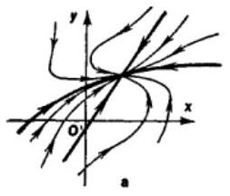
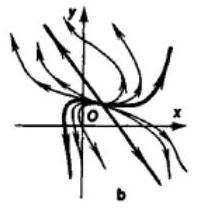
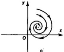
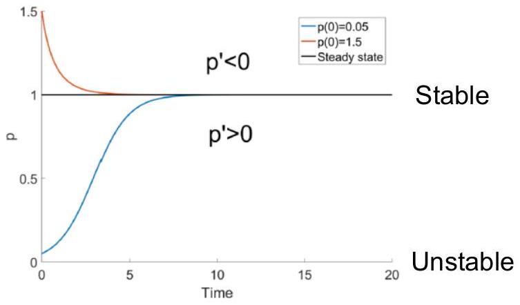
What does it mean that a steady state $u^{\ast }$ is (i) stable, (ii) asymptotically stable, and (iii) unstable?

• Stable: small perturbation from $u^{\ast }$ means that solution stays near $u^{\ast }$ for all time
• Unstable: small perturbation from $u^{\ast }$ leads to solution escaping from $u^{\ast }$
• Asymptotically stable: a solution that starts near enough to $u^{\ast }$ will converge to $u^{\ast }$ as $t\to \infty$

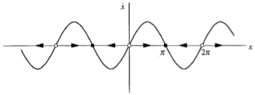
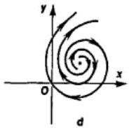
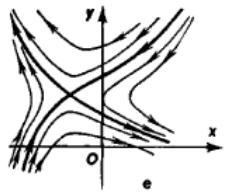
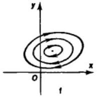
How are phase line plots used to provide insights into the dynamics of the solution?

$$u^{\prime }=f(u)$$

Where do we find mathematical models?

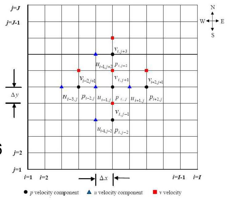
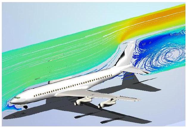
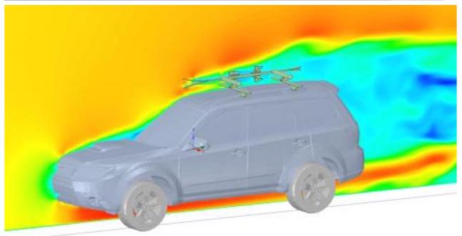
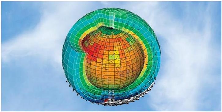
Fluid dynamics

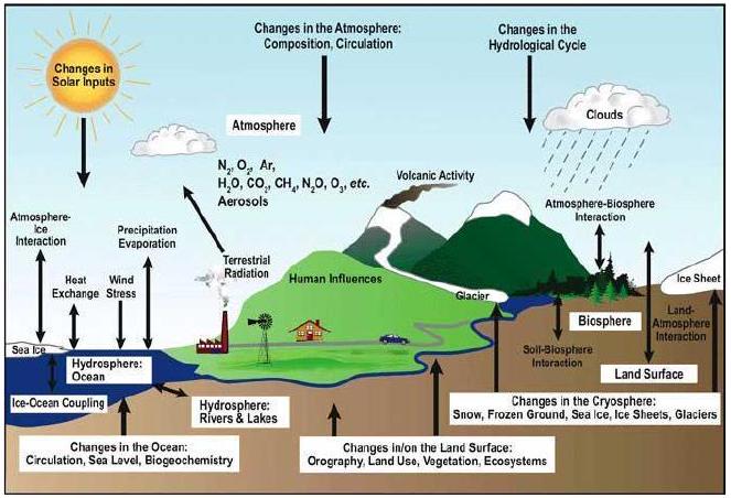
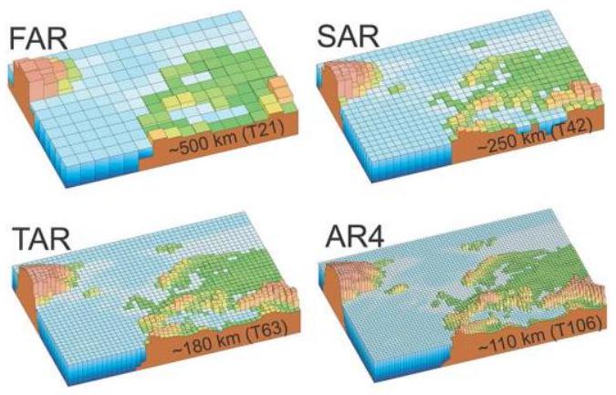
Climate modelling

Modelling covid and other infectious diseases

$$\begin{array}{rl}& \frac{ds}{dt}=-\beta si,\\ & \frac{di}{dt}=\beta si-\gamma i,\\ & \frac{dr}{dt}=\gamma i.\end{array}$$ $$R_0=\frac{\text{ infection rate }}{\text{ recovery rate }}=\frac{\beta si}{\gamma i}=\frac{\beta s}{\gamma }\approx \frac{\beta }{\gamma }$$

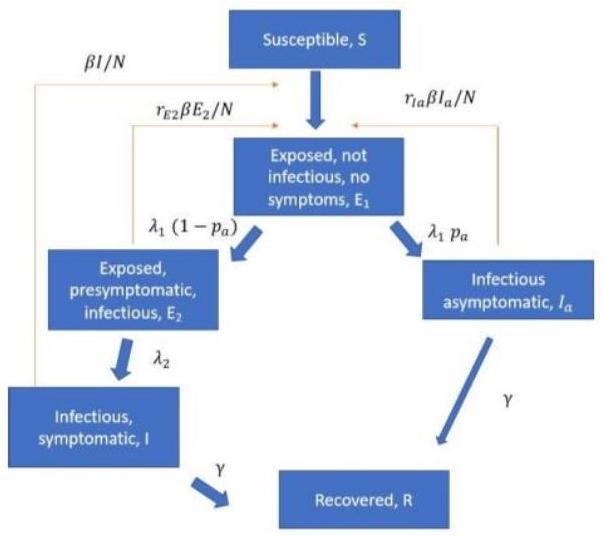
Source: https://www.fhi.no/en/id/infectious-diseases/coronavirus/coronavirus-modelling-at-the-niph-fhi/

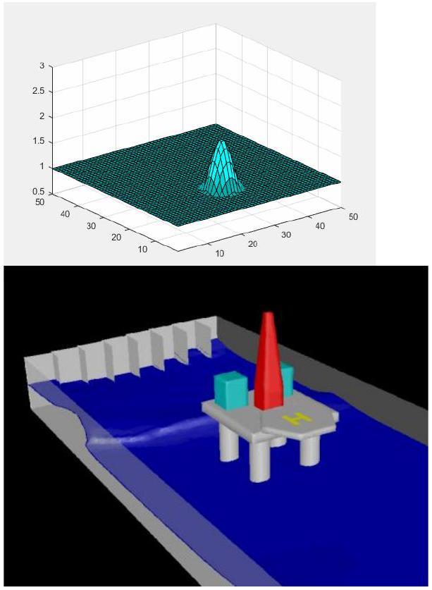
Physics engines for realistic physics in computer games

Alan M. Turing (1912-1954)

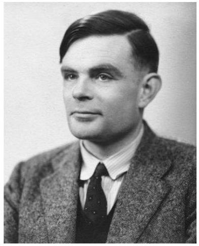
Enigma:

• Pioneer in computer science
• Developed a theory for biological pattern formation:

$$\begin{array}{rl}{u}_t& =u_{xx}+f(u,v),\\ v_t& =d{v}_{xx}+\underset{\text{Diffusion }}{\underbrace{g(u,v)}}.\end{array}$$

Pigment patterns in zebra fish: experiment and simulation

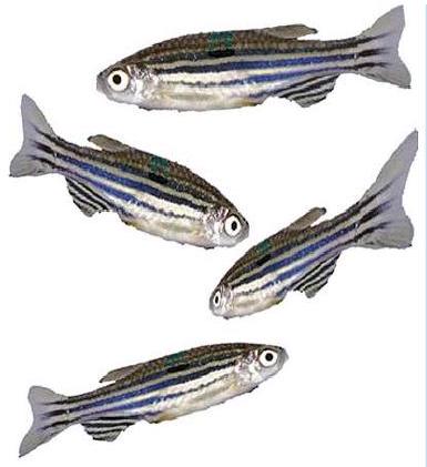
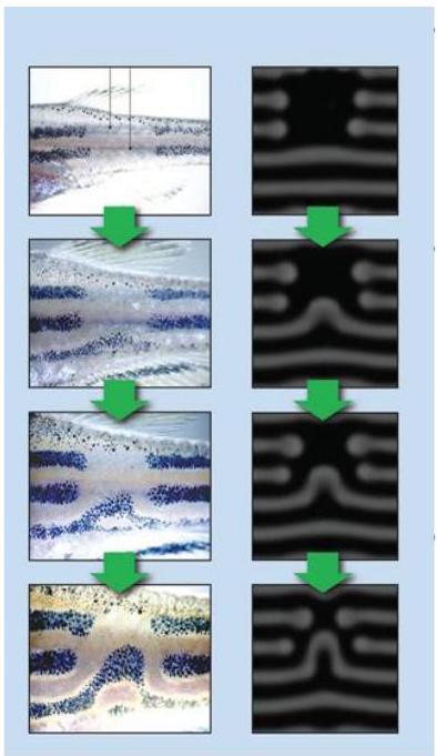Kondo & Miura, Science, 329, 2010. Showing laser ablation of pigment cells, migration of new cells, and a comparison of experiment with simulation.

Mathematical models in drug design

Mathematical Modelling to Guide Drug Development for Malaria Elimination — Hannah C. Slater, Lucy C. Okell, and Azra C. Ghani.

Data science, machine learning and AI

• Linear algebra
• Optimization
• Statistics and probability

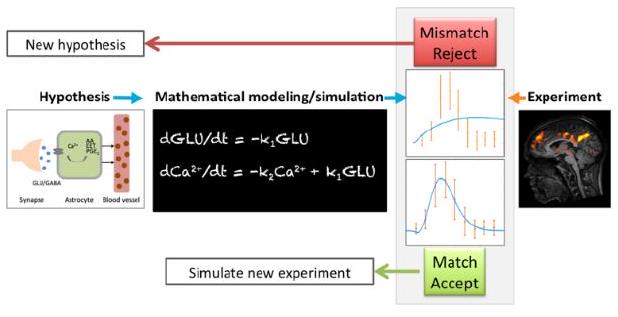
Why do we need mathematical models?

• To develop scientific understanding
  • e.g. hypothesis testing using the model as a testbed or laboratory
• To predict outcomes of experiments
  • e.g. perform experiments in silico to reduce costs and alleviate the need for animal experiments
• To test the effect of changes in a system
  • e.g. test the effect on model output of injecting a certain substance into the cell
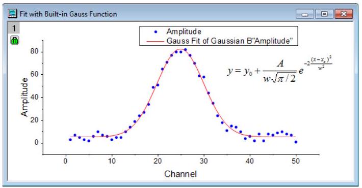
• To estimate parameters in a system
  • e.g. estimate parameter values by tuning them until the best fit between model output and empirical data is reached

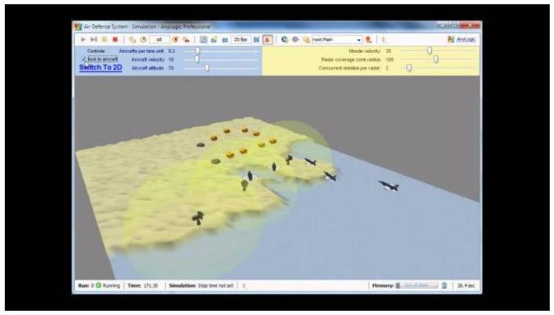
• To aid in decision making
  • e.g. describe various possible military scenarios using modelling and simulation. Generals may base their decisions on model outputs.

Different types of mathematical models

Types of models: Mechanistic vs empirical

• A mechanistic model uses available theoretical information, an empirical model does not
• The empirical model accounts quantitatively for changes associated with different conditions

6-1 Introduction To Empirical Models

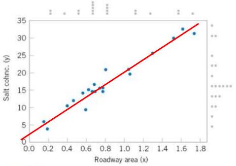
Figure 6-1 Scatter diagram of the salt concentration in surface streams and roadway area data in Table 6-1.

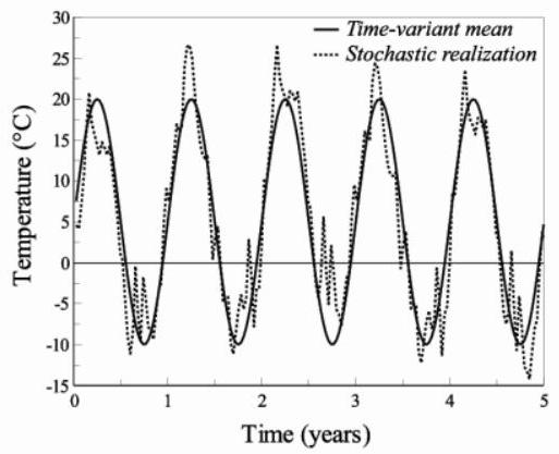
Types of models: Deterministic vs stochastic models

• Deterministic models ignore random variation
• Stochastic models account for randomness that often occurs in nature

Types of models: Dynamic vs static

• A dynamic model accounts for the system’s time-dependence
• A static model describes the state of the system in equilibrium

Types of models: Black box vs white box

• White box models are transparent, we know the details of the model and how the model produces predictions
• Black box models produce output that we can observe, but without knowing how it is produced
• (analogous to black box vs white box software)

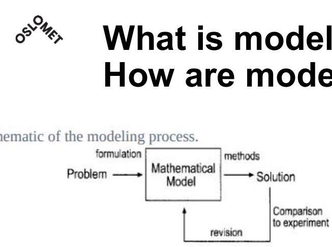
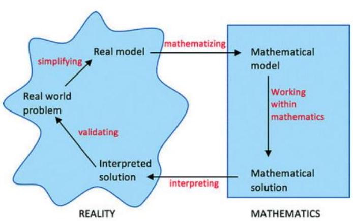
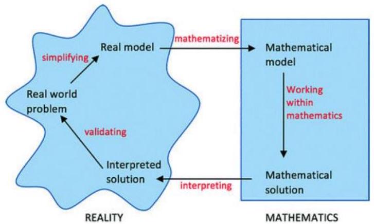
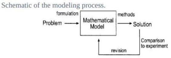
The modelling cycle

1. Describe the real-world model
2. Formulate the mathematical model
3. Calculate the solution of the model
4. Interpret the solution
5. Validate the model against real-world observations

Note: Progress is not necessarily sequential, and several iterations might be needed.

Compromises in mathematical modelling: how «good» should it be?

• First level of compromise: identify the most important parts of the system, include these in the model and exclude the rest.
  • Which parts are most important depends on the questions one wants to answer.
  • Examples:
    • Modelling a stone falling from a low height — air resistance can be justifiably neglected
    • Modelling a parachute — air resistance is of course crucial
• Second level of compromise: complexity of mathematical expressions.
  • Occam’s razor: the simplest mathematical expression is the best, since it requires the fewest assumptions (as long as the model maintains its realism).

Some examples of models

Second order differential equations

$$a{y}^{\prime \prime }+b{y}^{\prime }+cy=f(t).$$

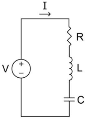
Newton’s 2nd law gives:

$$m{x}^{\prime \prime }+b{x}^{\prime }+kx=F(t).$$

Kirchhoff’s law gives:

$$L{Q}^{\prime \prime }+R{Q}^{\prime }+\frac{1}{C}Q=V(t).$$

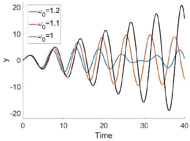
Resonance in second order differential equations

$$a=c=1,b=0,f(t)=\cos {\omega }_{0}t:$$

Population dynamics: the logistic equation

$$p^{\prime }=rp(1-p/K),$$

Steady states: $p=0,p=K$.

$$p(t)=\frac{p_{0}K}{p_0+\left(K-p_0\right)e^{-rt}},$$

Population dynamics: predator–prey interactions

$$\begin{array}{rl}{x}^{\prime }& =ax-bxy,\\ y^{\prime }& =cxy-dy,\end{array}$$

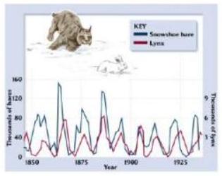
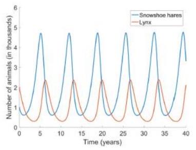
Steady states: $\left(x^{\ast },y^{\ast }\right)=(0,0)$ and $\left(x^{\ast },y^{\ast }\right)=\left(\frac{d}{c},\frac{a}{b}\right)$.

Alan L. Hodgkin

Andrew Huxley

Mathematical modelling in physiology

Denis Noble

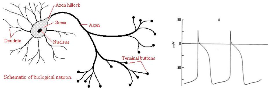
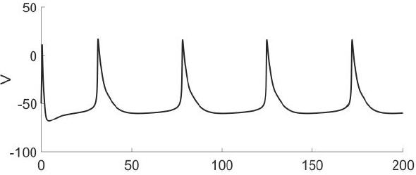
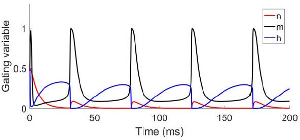
The Hodgkin–Huxley model

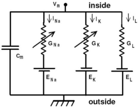
Gating $\Rightarrow$ conductances of K- and Na-channels depend on $V$ $\Rightarrow$ interesting dynamics.

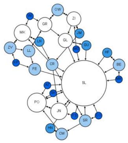
Information flow through neurons:

The Hodgkin–Huxley model

Differential equations

Why consider differential equations?

Describes dynamics in terms of rate of change.

«Solvable» ODEs

Linear and homogeneous first order ODEs:

$$a{y}^{\prime }+by=0$$

Separable ODEs:

$$f(y)y^{\prime }=g(t)$$

First order general linear ODEs:

$$y^{\prime }+p(x)y=q(x)$$

Second order linear ODEs with constant coefficients:

$$a{y}^{\prime \prime }+b{y}^{\prime }+cy=f(x)$$

Problems

• Solve the ODEs:
  • $y^{\prime }=y{x}^2$
  • $\left(1+x^2\right)y^{\prime }+y^2=0$
  • $y^{\prime }+2y=1$
• Solve the initial value problems:
  • $y^{\prime }=x\sqrt{y},y(2)=4$
  • $y^{\prime }+xy=0,y(0)=1$

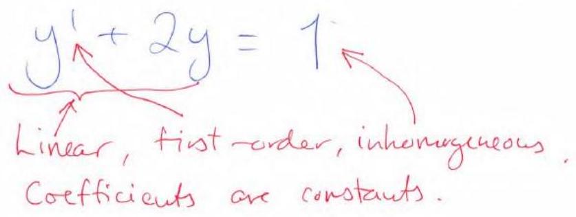
Worked example: $y^{\prime }+2y=1$

This is a linear, first-order, inhomogeneous ODE with constant coefficients.

General solution:

$$y=y_H+y_P$$

where $y_H$ is the general solution of the corresponding homogeneous ODE and $y_P$ is a particular solution.

$y_H$ is the general solution of:

$$\begin{array}{rl}{y}^{\prime }+2y& =0\\ \iff y^{\prime }& =-2y\\ \iff y_H& =C{e}^{-2t}\end{array}$$

$y_P$ is a particular solution of $y^{\prime }+2y=1$. We observe that $y_P=\frac{1}{2}$ is a particular solution. Therefore:

$$y=y_H+y_P=C{e}^{-2t}+\frac{1}{2}$$

Worked example: $y^{\prime }=x\sqrt{y},y(2)=4$

This is an initial value problem (IVP): the ODE $y^{\prime }=x\sqrt{y}$ plus the initial condition $y(2)=4$. The ODE is separable:

$$y^{\prime }=x\sqrt{y}\iff \frac{1}{\sqrt{y}}{y}^{\prime }=x$$

Integrating:

$$\int \frac{1}{\sqrt{y}}dy=\int xdx\Rightarrow 2\sqrt{y}=\frac{1}{2}{x}^2+C_1\Rightarrow \sqrt{y}=\frac{1}{4}{x}^2+C$$ $$\Rightarrow y={\left(\frac{1}{4}{x}^2+C\right)}^2\text{(general solution)}$$

Applying $y(2)=4$:

$$\begin{array}{rl}& (\underset{=1}{\underbrace{\frac{1}{4}\cdot 2^2}}+C{)}^2=4\\ & (1+C{)}^2=4\\ & C=1\text{ and }C=-3\end{array}$$

Two solutions:

$$\begin{array}{rl}& y={\left(\frac{1}{4}{x}^2+1\right)}^2\\ & y={\left(\frac{1}{4}{x}^2-3\right)}^2\end{array}$$

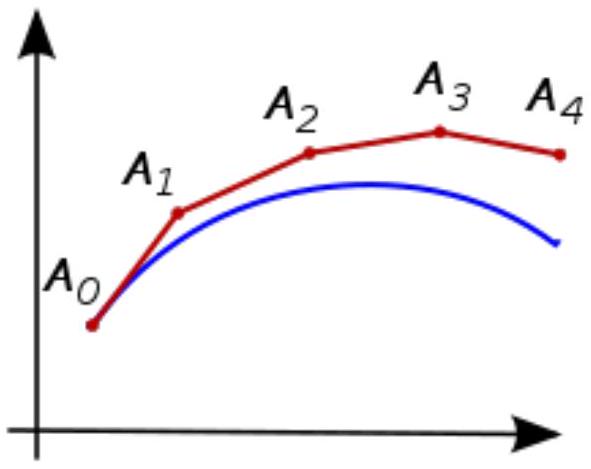
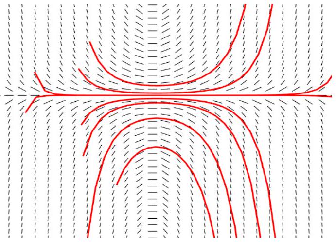
Slope fields

Slope field (direction field)

• Differential equation: $y^{\prime }=F(x,y)$
• The derivative $y^{\prime }$ is the slope of the tangent of the solution curve
• A slope field is defined by the magnitude of the derivatives, indicated by short straight lines
• An ODE has (most often) infinitely many solutions

The initial value problem

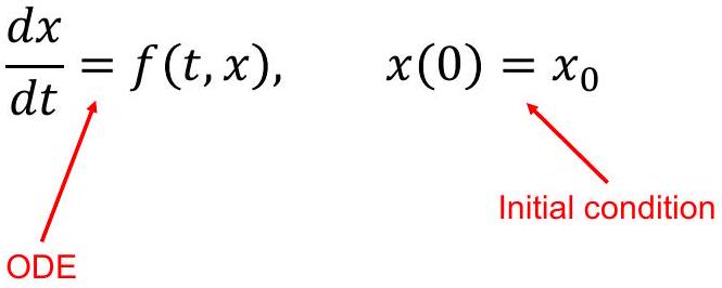
Normally one solution per initial value. (Shown: solution with initial condition $y(0)=0.2$.)

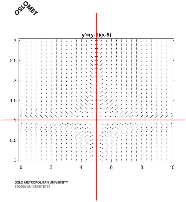
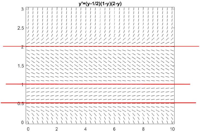
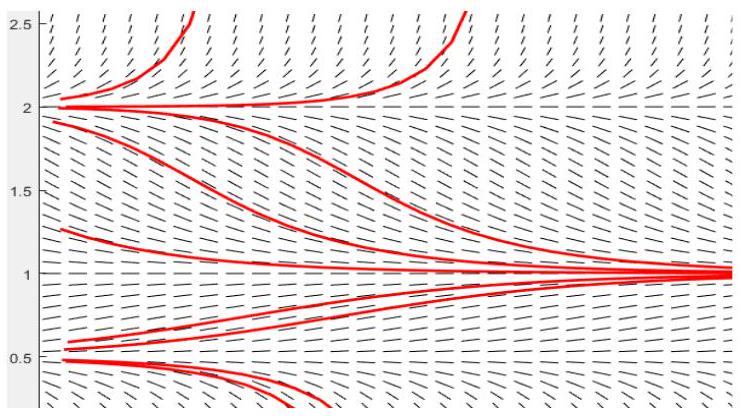
Slope fields, examples

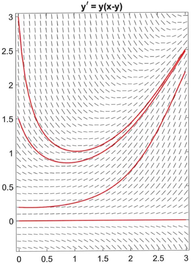
Slope fields, problem

• Sketch the slope field of the ODE

$$y^{\prime }=y/x$$

(calculate $y^{\prime }$ for a number of points in the coordinate system)

• What kind of solutions do we have?

Solving $y^{\prime }=y/x$

As a separable ODE:

$$\begin{array}{c}\frac{1}{y}{y}^{\prime }=\frac{1}{x}\\ \int \frac{1}{y}dy=\int \frac{1}{x}dx\\ \ln |y|=\ln |x|+C\\ |y|=K_1|x|\end{array}$$

With $K=\pm K_1$, the general solution is $y=Kx$.

Using the integrating factor:

$$y^{\prime }=\frac{y}{x}\iff y^{\prime }-\frac{1}{x}y=0$$ $$\text{Integrating factor}=e^{-\int \frac{1}{x}dx}=e^{-\ln |x|}={\left(e^{\ln |x|}\right)}^{-1}=|x{|}^{-1}$$

Assume $x>0$:

$$\frac{1}{x}{y}^{\prime }-\frac{1}{x^2}y=0\iff {\left(\frac{1}{x}y\right)}^{\prime }=0\iff \frac{1}{x}y=K\iff y=Kx$$