PENG9570 Final Report: 04 Results and Discussion

About

Writing Project:: PENG9570 Course Project - Writing Project - VIBE Draft Index:: Drafts - PENG9570 Course Project - VIBE Outline Partner:: 05 - Results and Discussion - Outline 1 Previous Draft:: 04 - Results and Discussion - Draft 6 - HUMAN Role:: Final report draft adapted from Overleaf final modifications

4. Results and Discussion

4.1 Baseline Configuration and Changing Forcing Function

In the decomposition $\bar{u}-u^{\star }=(\bar{u}-u_h)+(u_h-u^{\star })$, the first term is the NeuroFEM solver contribution and the second is the FEM discretization contribution. The three reported metrics are:

$${\epsilon }_{\mathrm{res}}=\frac{\Vert A_{\mathrm{sys}}\bar{u}-M{f}_1\Vert }{\Vert M{f}_1\Vert },{\epsilon }_{\mathrm{ana}}=\frac{\Vert \bar{u}-u^{\star }\Vert }{\Vert u^{\star }\Vert },{\epsilon }_{\mathrm{slv}}=\frac{\Vert \bar{u}-u_h\Vert }{\Vert u_h\Vert },$$

where ${\epsilon }_{\mathrm{res}}$ is the relative residual, ${\epsilon }_{\mathrm{ana}}$ compares NeuroFEM against the analytic solution, and ${\epsilon }_{\mathrm{slv}}$ compares NeuroFEM against the direct solver (scipy.solve_system_sparse_direct).

For the constant forcing case $f_1$, the time-averaged readout $\bar{u}$ over the last $T=10^4$ pre-switch timesteps gives the results in Table 1.

Table 1: Baseline results for $N_{\mathrm{interior}}=1218$, NPM $=16$, $|\Gamma |=2^{-6}$.

Symbol	Quantity	Value
${\epsilon }_{\mathrm{res}}$	Relative residual	$1.287\times 10^{-3}$
${\epsilon }_{\mathrm{ana}}$	NeuroFEM vs. analytic	$1.924\times 10^{-3}$
${\epsilon }_{\mathrm{slv}}$	NeuroFEM vs. direct solver	$4.1\times 10^{-5}$

These match the article’s main-text definition of the relative residual, $\Vert \mathbf{b}-A\mathbf{x}\Vert /\Vert \mathbf{b}\Vert$, rather than the per-mesh-node residual $r=\frac{1}{N_{\mathrm{mesh}}}\Vert \mathbf{b}-A\mathbf{x}\Vert /\Vert \mathbf{b}\Vert$ plotted in the article’s Fig. 2c—d. Comparing ${\epsilon }_{\mathrm{res}}$ against those panels therefore requires dividing by $N_{\mathrm{mesh}}=1218$.

The error ratio between solver methods ${\epsilon }_{\mathrm{ana}}/{\epsilon }_{\mathrm{slv}}\approx 47$, meaning the NeuroFEM solver is nearly fifty times closer to the direct discrete FEM solution than to the analytic solution.

The forcing-switch experiment tests a different property. During the first half of the run, the readout converges toward the solution for $f_1$. At step 25,000 the bias changes to bias_f2; the same recurrent weights then relax toward the solution for $f_2$ (see Fig. 2).

This confirms the SNN’s ability to adapt flexibly and online without requiring a learning step or additional updates to the network hyperparameters; forcing functions can be solved by changing biases rather than reconstructing the network.

The cached NPM $=8$ parameter file provides a secondary check on population size. This is not a full parameter study, but we replicate similar results: fewer neurons per mesh node increase readout noise floor and worsen direct-solver comparison accuracy.

Fig. 2: Our reproduction of Fig. 1e

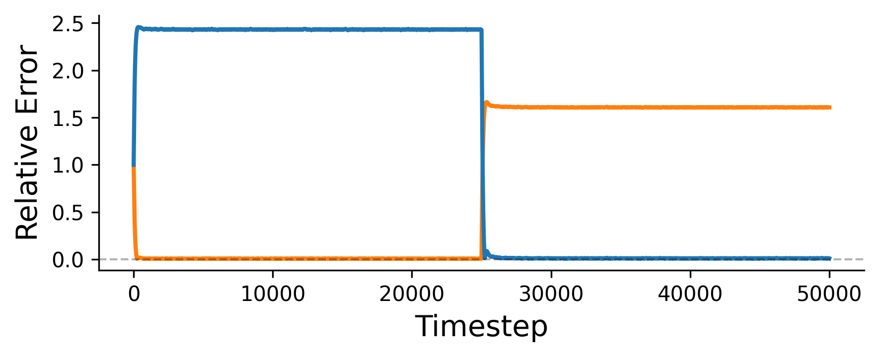Our reproduction of Fig. 1e from the original paper. The activity of a NeuroFEM circuit constructed to solve the Poisson equation on a disk flows to the solutions with respect to two different right-hand sides $f_1$ and $f_2$. The right-hand side switches from $f_1$ to $f_2$ at timestep 25,000.

4.2 Parameter Sweep

We replicate the parameter sweep test for the NPM values, number of mesh nodes $N_{\mathrm{interior}}$, and readout magnitude $|\Gamma |$, then compare the results against the analytic and standard solvers. We exclude the largest mesh case ($N_{\mathrm{interior}}=12079$) as it is not computationally tractable to us. We recreate the results seen in Fig. 2(b,c,d) of Theilman and Aimone (2025) \cite{theilmanSolvingSparseFinite2025}, shown here in Fig. 3.

Fig. 3: Neuromorphic finite element algorithm parameter sweep (original)

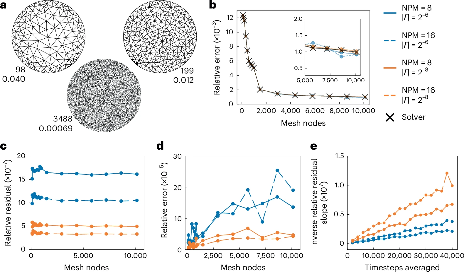Taken from Theilman and Aimone (2025) \cite{theilmanSolvingSparseFinite2025}. We reproduce panels b, c, and d. (a) NeuroFEM benchmark: Poisson equation on a disk with Dirichlet boundary conditions. (b) Relative error with respect to the analytic solution as a function of mesh resolution for NeuroFEM and a conventional solver. (c) Relative residual of the linear system per mesh point; constant as a function of mesh nodes; improved by increasing NPM or decreasing $|\Gamma |$. (d) Relative error between NeuroFEM and the conventional solver. (e) Relative residual improves linearly with the number of averaged readout timesteps.

The conventional FEM baseline error ${\epsilon }_{\mathrm{ana}}$ decreases from approximately $1.19\times 10^{-2}$ at $N_{\mathrm{interior}}=118$ to approximately $1.09\times 10^{-3}$ at $N_{\mathrm{interior}}=6503$ (Fig. 4). Across all tested mesh sizes, NeuroFEM matches the conventional solver results closely. For example, at $N_{\mathrm{interior}}=377$, NeuroFEM errors lie between $[8.542,8.571]\times 10^{-3}$ while the conventional solver gives $8.561\times 10^{-3}$. Additionally, we see no divergence with respect to the readout magnitude until $N_{\mathrm{interior}}=12079$, where fewer NPM regimes fail to integrate the larger mesh input.

Fig. 4: Relative error with respect to the analytic solution

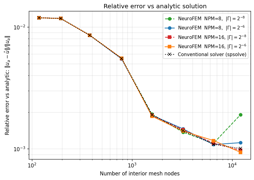Our reproduced results for the relative error ${\epsilon }_{\mathrm{ana}}$ with respect to the analytic solution as a function of mesh resolution, for NeuroFEM and the conventional solver. For comparison see Fig. 3b.

Measuring ${\epsilon }_{\mathrm{res}}$ against $N_{\mathrm{interior}}$ appears to directly relate to magnitude, with low-magnitude parameter regimes scoring better, then secondarily with respect to NPM, where higher NPM scores better within their magnitude bands (Fig. 5). This matches the expected outcomes seen in the original article (Fig. 2c of the original article).

Fig. 5: Relative residual per mesh point

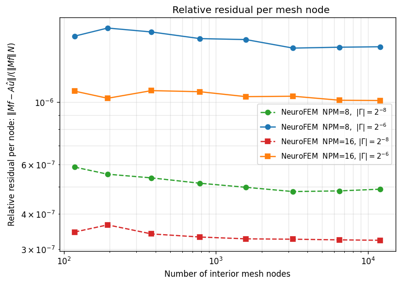Our reproduced results for the relative residual ${\epsilon }_{\mathrm{res}}$ of the linear system per mesh point as a function of the number of mesh nodes. The relative residual is improved by increasing NPM and/or decreasing $|\Gamma |$. For comparison see Fig. 3c.

In Fig. 6 we compare the relative error between NeuroFEM and the conventional solver ${\epsilon }_{\mathrm{slv}}$, where we can observe more variation between methods albeit slight, with the low-magnitude, small NPM performing the worst at $1.90\times 10^{-3}$. Surprisingly, our results do not match our expected outcomes: the best performing regime is a high-NPM, low-magnitude one, whereas in the original article both low-magnitude regimes consistently scored better than the high-magnitude regimes (Fig. 3). This may be due to an error in our interpretation of the code or possibly a difference of hardware environments. Further investigation will be required at a later time.

Fig. 6: Relative error between solvers

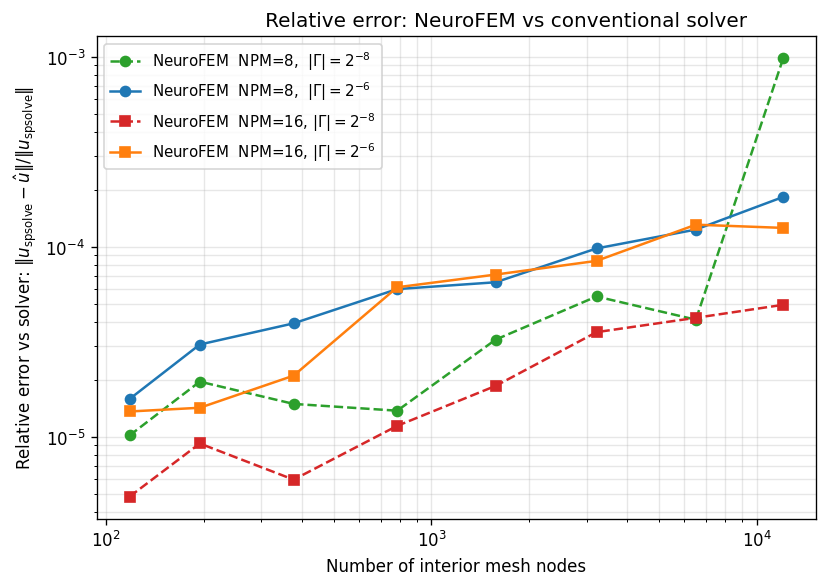Our reproduced results for the relative error ${\epsilon }_{\mathrm{slv}}$ between NeuroFEM and the conventional solver. For comparison see Fig. 3d.