PENG9570: Course summary
Questions and suggested answers

Mathematical modelling
What is a mathematical model?
- a description of a system using mathematical concepts and language.
Why do we need mathematical models?
- To develop scientific understanding
- To predict outcomes of experiments
- To test the effect of changes in a system
- To estimate parameters in a system
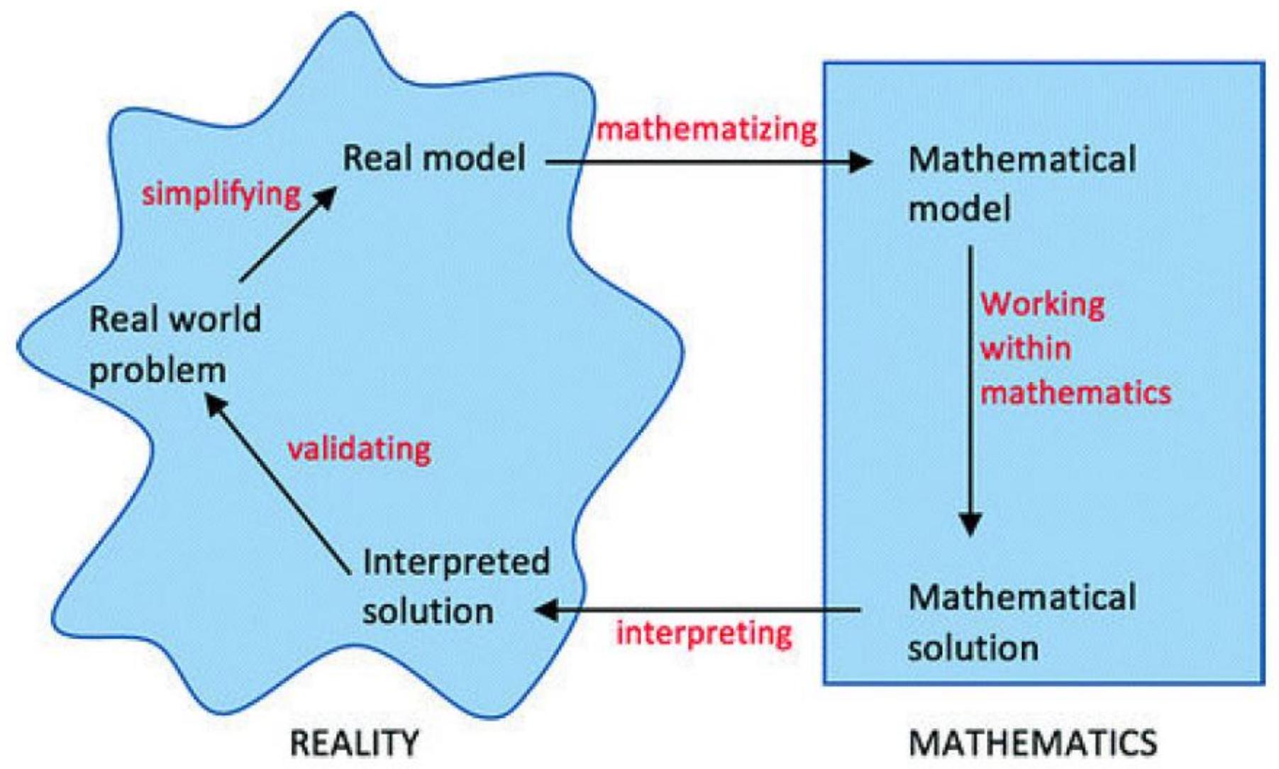
Describe the stages of the modelling cycle
ODEs and systems of ODEs
What is a differential equation and what is an initial value problem?
- Differential equation:
- Initial value problem:
- Differential equation plus initial values for and, possibly, some of its derivatives
- Example:
What is the steady state (or critical point or equilibrium) of a first order differential equation?
- In one-variable models :
The value such that the derivative is zero:
- In two-variable models :
The point such that the derivatives are zero: and
What does it mean that a steady state is (i) stable, (ii) asymptotically stable and (iii) unstable?
- Assume is a steady state
- Stable: small perturbation from has little effect (solution stays near )
- Unstable: small perturbation from has large effect (solution escapes from )
- Asymptotic stability: a solution that starts near enough to will converge to as
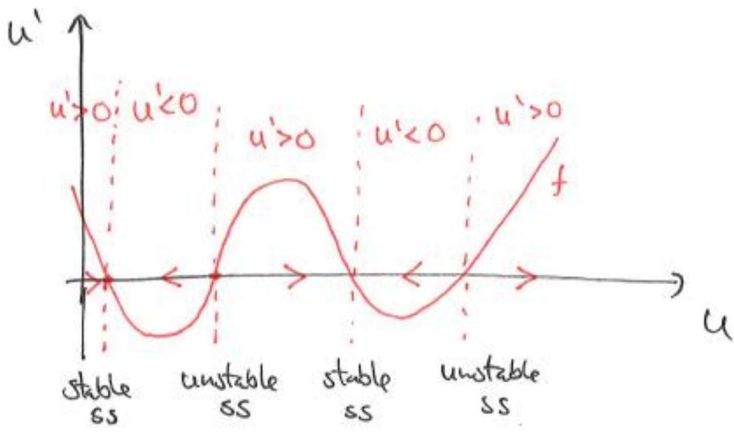
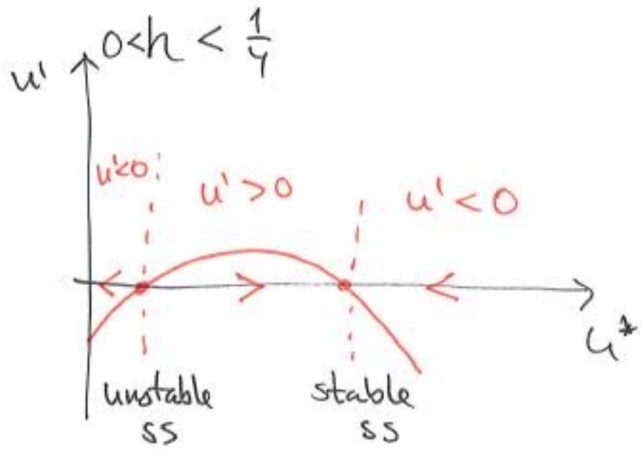
How are phase line plots used to provide insights into the dynamics of the solution?
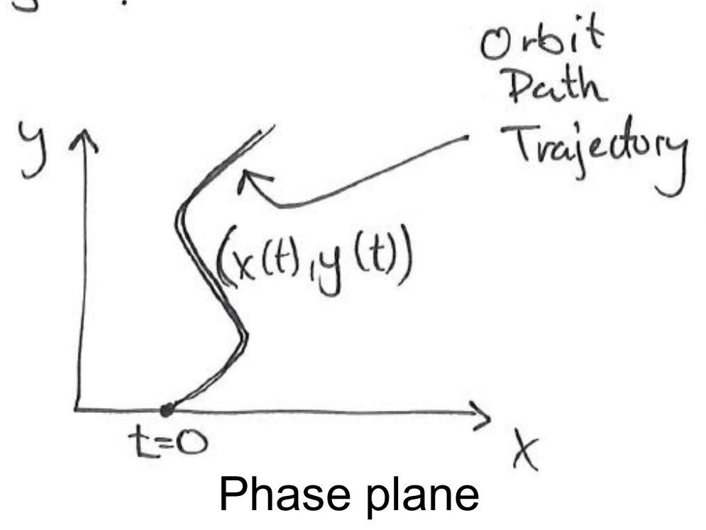
Two-dimensional dynamical systems
Solution: - functions of time
Solution Curres:

What is the linearization of an ODE system?
In what way does the linearization inform us about the nonlinear system?
Assumption: critical point in .
Linearisation: (due to
is the Jacobian.
Dynamics can be deduced from eigenvalues and eigenvectors of Jacobian
Name the four types of critical points and relate them to the eigenvalues of the coefficient matrix (linear system) or of the Jacobian (nonlinear system).


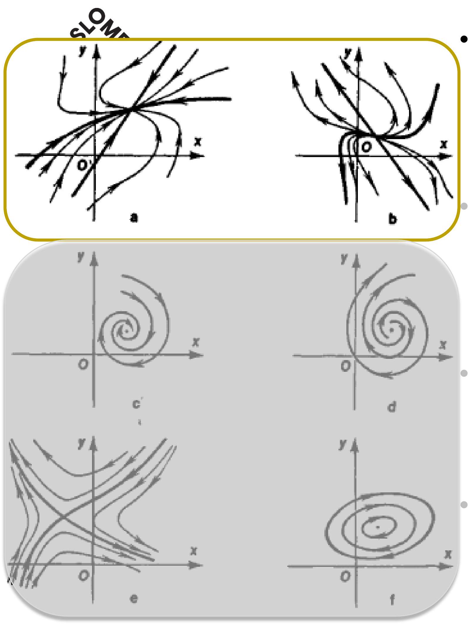
Node
- Two real eigenvalues of same sign
- Stable if both eigenvalues are negative
- Unstable if both eigenvalues are positive
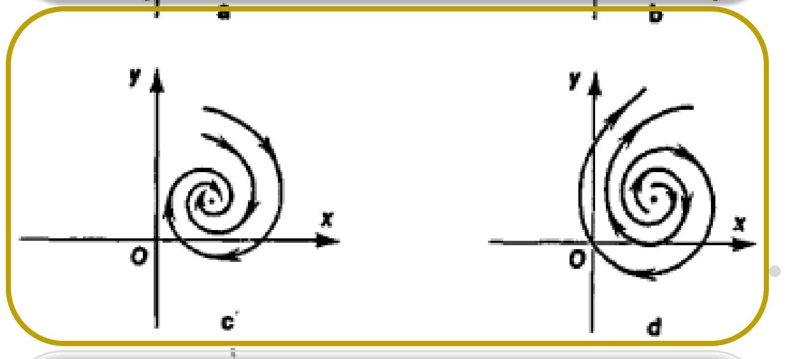
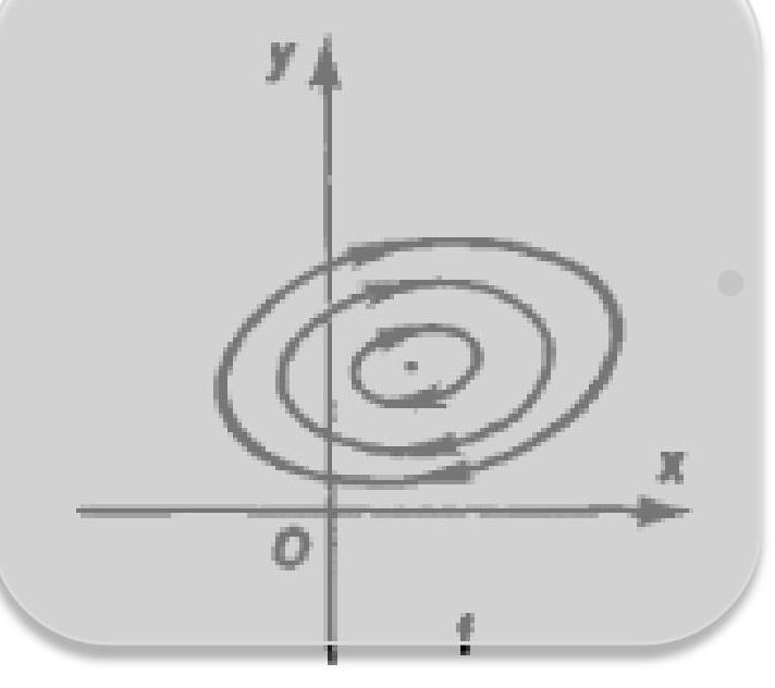
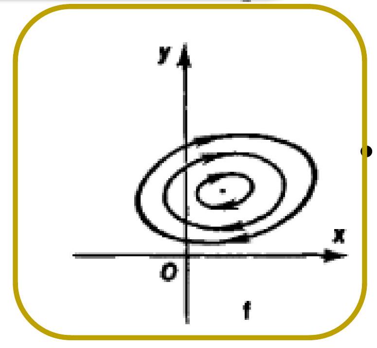
Spiral
- Complex eigenvalues
- Stable if for both eigenvalues
- Unstable if for both eigenvalues
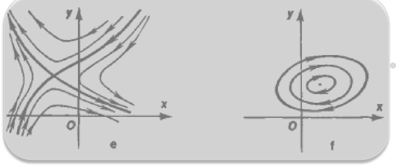
Saddle
- Two real eigenvalues, one positive and one negative
Center
- Two purely imaginary eigenvalues

Node
- Two real eigenvalues of same sign
- Stable if both eigenvalues are negative
- Unstable if both eigenvalues are positive
Spiral
- Complex eigenvalues
- Stable if for both eigenvalues
- Unstable if for both eigenvalues
Saddle
- Two real eigenvalues, one positive and one negative
Center
- Two purely imaginary eigenvalues
- Two real eigenvalues of same sign
- Stable if both eigenvalues are negative
- Unstable if both eigenvalues are positive
Spiral


- Two real eigenvalues, one positive and one negative
Center
- Two purely imaginary eigenvalues

- Two real eigenvalues of same sign
- Stable if both eigenvalues are negative
- Unstable if both eigenvalues are positive
Spiral
- Complex eigenvalues
- Stable if for both eigenvalues
- Unstable if for both eigenvalues
Saddle

- Two real eigenvalues, one positive and one negative
Center
- Two purely imaginary eigenvalues
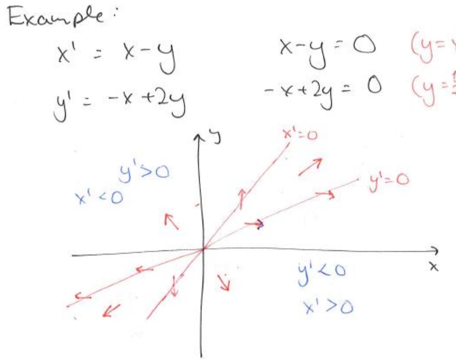
What is a nullcline?
Explain how nullclines and vector fields are used to provide information on solution orbits
The nullclines of a system are the curves obtained when the derivatives and are set equal to zero:
What is a bifurcation and what is depicted in a bifurcation diagram?
- Assume there is a parameter (the bifurcation parameter) in our ODE system
- We have a bifurcation point at the value of this parameter where a new type of solution emerges
- A bifurcation diagram shows the possible steady state values (stable and unstable) of a system as a function of a bifurcation parameter
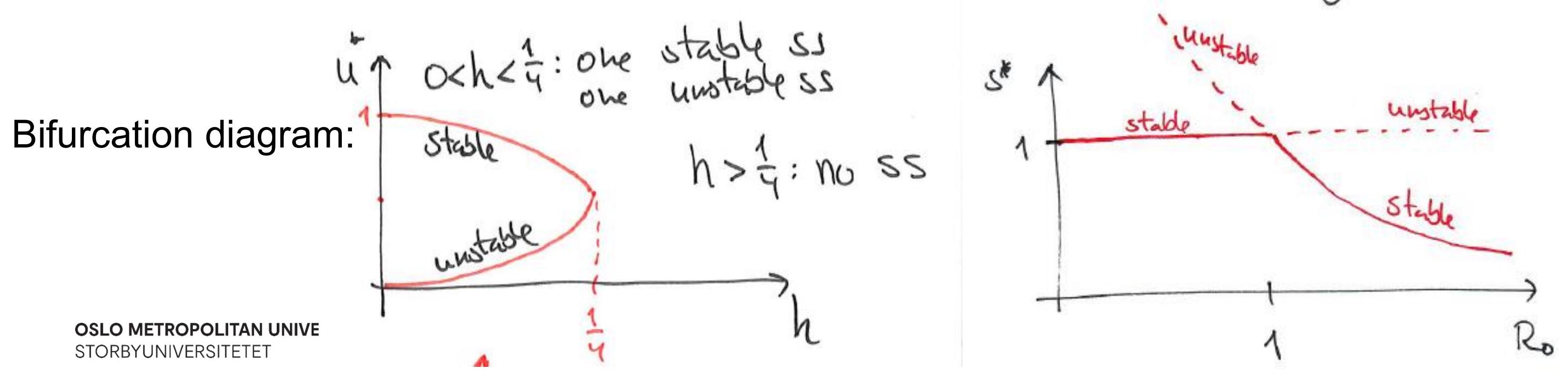
- I want- [ ] I want to know what is being plotted here on the bifurcation diagram
Existence and uniqueness theorem for IVPs: Define the integral form and the Picard iteration
Integral form of IVP:
- [?] IVP?
The Picard iteration
Sequence of approximations to integral form:
- [?] No idea what this is supposed to mean. It’s the same formula but with some variable changed, but not explained
If the sequence converges to a limit function is the solution of the IVP.
Existence and uniqueness theorem for IVPs: Define Cauchy sequence and completeness
Cauchy sequence
A sequence where the elements come arbitrarily close to each other when the sequence numbers are sufficiently large. Mathematically, for every positive , there is an integer such that for all ,
Completeness
A set is said to be complete provided that all Cauchy sequences of elements in the set converge to an element in .
Thus, establishing that a sequence of elements belonging to a complete set is Cauchy, we can conclude that the sequence will converge to a limit in .
Formulate the existence and uniqueness theorem
Given the IVP
Providing that is continuous and differentiable ( ),
- What does this mean? Specifically C_1 and E there exists such that there exists a unique solution in . (Existence and uniqueness)
Give a sketch of the proof of existence
- SHIT this looks very very important
- Construct sequence of approximate solutions using Picard iteration.
- Show that this sequence is Cauchy within the space of continuous functions (depends on the differentiability of ).
- Since is complete, then the sequence must converge to an element within .
- This limit is the solution and existence is established.
Numerical methods for IVPs
Why do we need numerical methods to solve differential equations?
- In general it is not possible to find an analytical solution
- The differential equations need to be translated into equations that can be solved on a computer
How do we write an initial value problem on integral form?
Integrating the initial value problem (IVP)
from to we obtain
The integral is in general evaluated numerically to obtain a numerical solution of the IVP.
Use numerical integration to explain the accuracy of Euler’s method
- Use numerical integration to explain the accuracy of Euler’s method
The integral is evaluated numerically (here ):
- Euler’s method: Riemann left sum (Order - method is order )
- Not clear what “order h” means
Euler’s steps
I think this is a iterative method. I’ve seen “Euler Steps” mentioned elsewhere. As in a number of timesteps to be integrated over piecewise.
Use numerical integration to explain the accuracy of Heun’s method
- Use numerical integration to explain the accuracy of Heun’s method
The integral is evaluated numerically (here ):
- Heun’s method: Trapezoidal rule (Order - method is order )
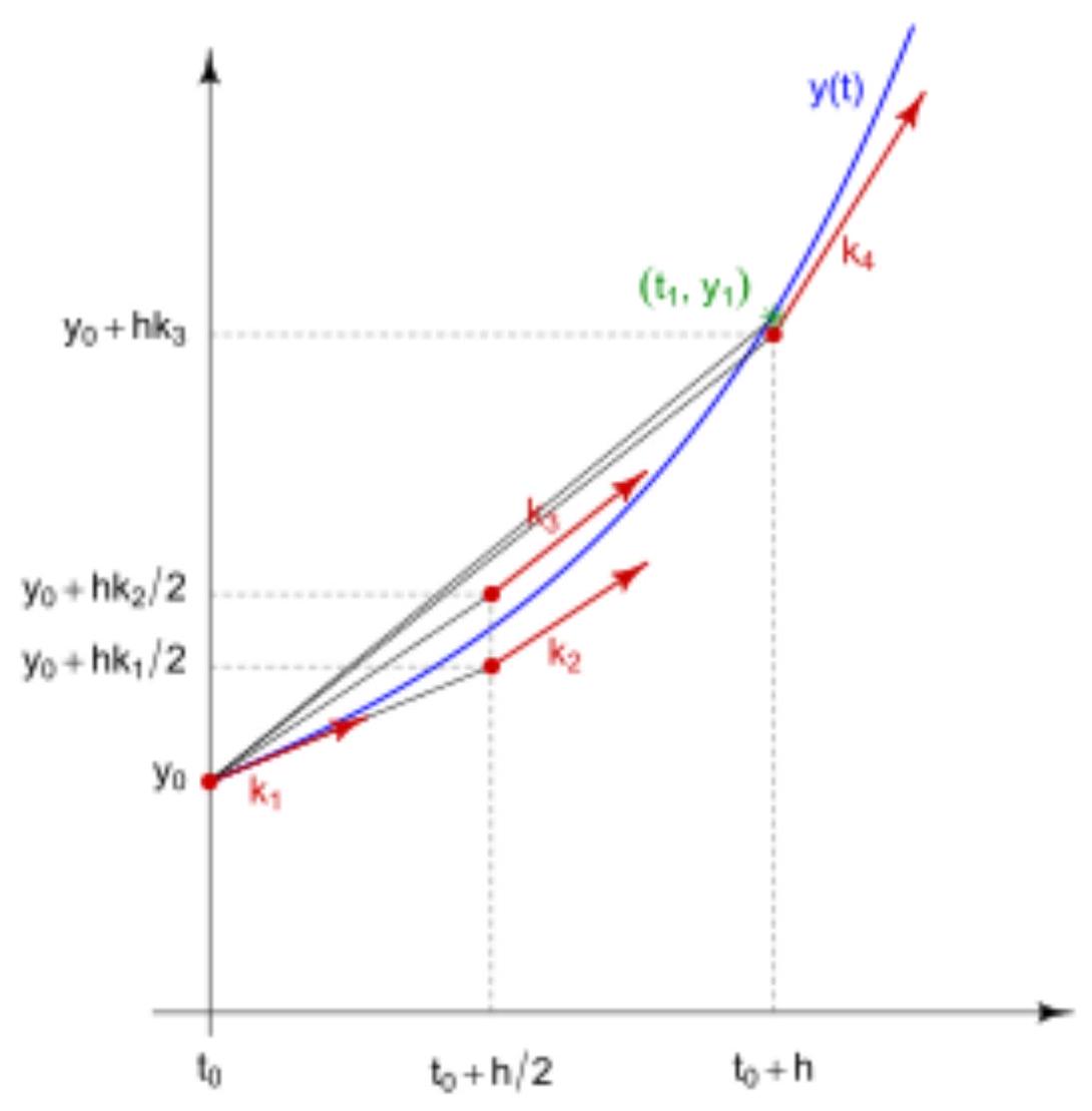
Use numerical integration to explain the accuracy of Runge-Kutta’s 4th order method
The integral is evaluated numerically (here ):
- Runge-Kutta’s 4th order method: Simpson’s rule (Order method is order )
- Estimate for solution at time step is obtained by stepwise estimation of slopes at time steps and
PDEs
What is the difference between ODEs and PDEs ?
ODEs: solution is function of one variable
PDEs: solution is function of two or more variables and partial derivatives of more than one of the variables are part of the equation
Examples:
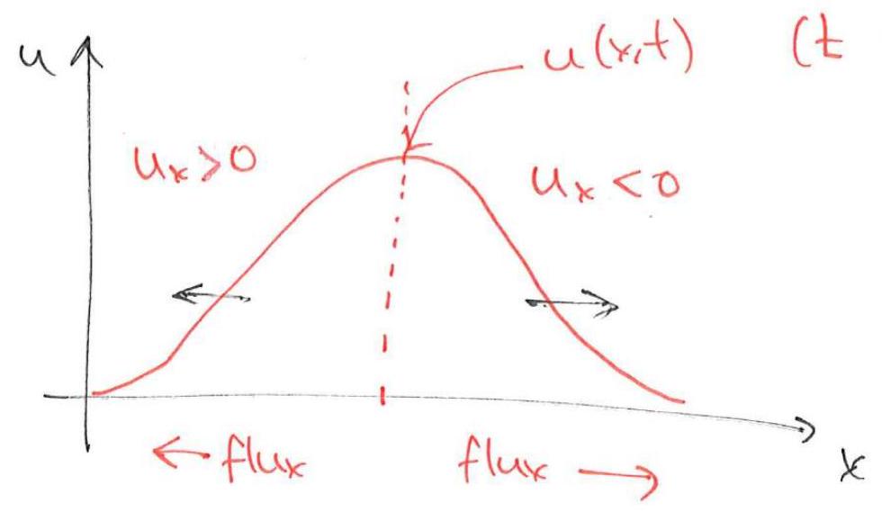
How is the diffusion PDE derived from a conservation law?
: Quantity of a substance : flux of substance (or heat flux) : production rate Conservation law in integral form is obtained by requiring the following (on interval ):
Rate of change of amount of substance what comes in - what goes out + rate of production
This, in turn, gives the conservation law in differential form :
Diffusion (and heat): (Fick’s law) .
What do we mean by linearity and superposition of solutions?
PDEs are often written using operators. Example:
The operator is linear when
For homogeneous problems , super-positions of solutions are also solutions:
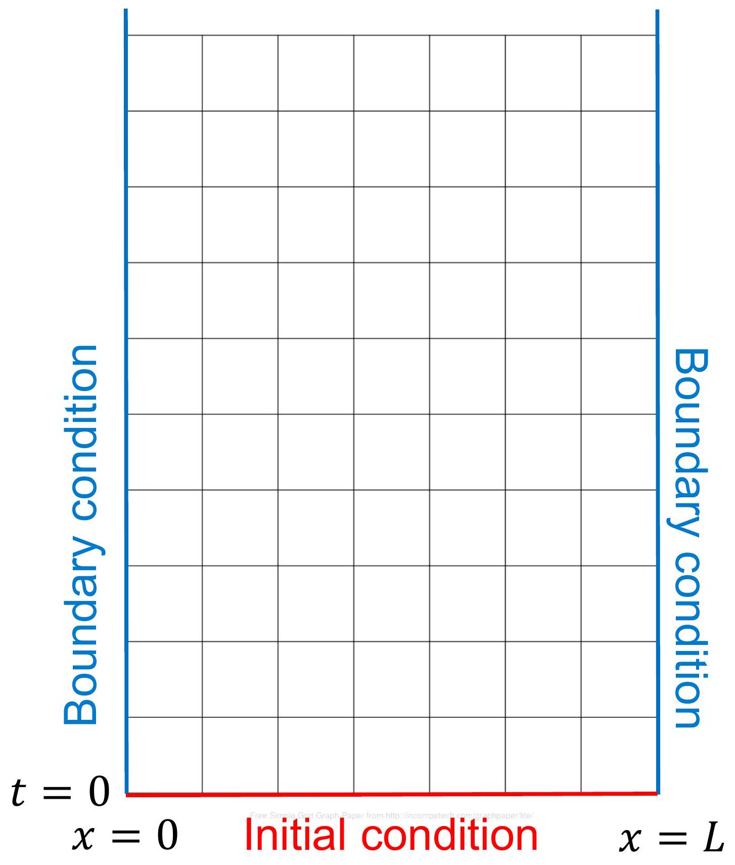
What is an initial boundary value problem
(IBVP) for a PDE?
Example: 1D diffusion PDE with initial and boundary conditions
Prove uniqueness of the IBVP
Assume two solutions and . Then solves
- Define the energy integral
- Show (without too much detail) by differentiation and integration by parts that must be zero
- This proves that
- Uniqueness is proven!
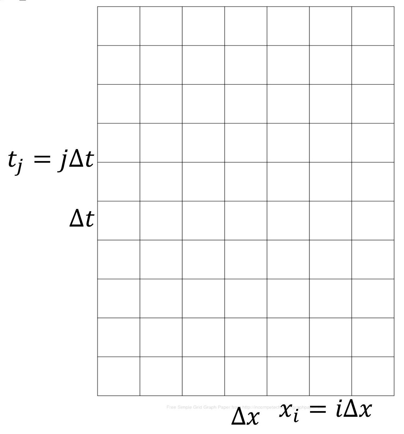
Numerical methods for IBVPS
How are partial derivatives approximated by finite difference expressions?
Typical approximations:
Let . Then,
Explain the explicit scheme
PDE: . Let . Then,
That is,
where
Derive the stability criterion in terms of for the explicit scheme
Explicit scheme:
where
Scheme is stable if eigenvalues of are less than 1 in absolute value. Eigenvalues are ( are eigenvalues of ).
must hold for all values of including :
What is the difference between explicit and implicit schemes?
- Explicit scheme:
forward time derivative (forward Euler)
- Implicit scheme:
backward time derivative (backward Euler)
Show that the implicit scheme is stable for all values of
- Implicit scheme is
- Eigenvalues of are .
- Scheme is stable!
What is the difference between the Crank-Nicolson scheme and the previous schemes?
Same as implicit method, except that is approximated with the average of approximations at time steps and :
Advantage: the Crank-Nicolson scheme is more accurate than the other schemes when evaluating at points : error at his point is
Show that the Crank-Nicolson scheme is stable
- Crank-Nicolson scheme is of the form
- Eigenvalues of are .
⇒ eigenvalues are .
- Scheme is stable!
The Schrödinger equation
- How can the numerical methods previously considered be applied to solve this PDE ?
- Quite straightforward, with some adjustments (e.g. solutions of the Schrödinger equation are generally complex)
- How can this PDE be rewritten as a coupled system of ODEs?
- Approximate and solve the resulting large ODE system
- Explain how the solution is interpreted as a probability density
- The integral is probability of a particle being located in